Value investing is an investment philosophy that has been extensively discussed and examined at least since the days of Ben Graham, who popularized it as a discipline in the 20s and 30s. While there are some who are dismissive of its advantages as a long-term strategy, the historical evidence is compellingly clear: Cheap stocks beat expensive stocks over time (see our simulation study as an example). Of course, on a relative performance basis, value can be excruciatingly painful.
In academia, scholars have gone to great lengths to determine which processes and variations on the value philosophy are most effective. Yet the high-performance strategies identified in academic research are typically not available in the real-world marketplace. There are a number of reasons why this is the case, but they typically boil down to career-risk incentives, scale, and branding. A common mistake by financial service consumers is to focus solely on fees and branding, but little on the process. However, while branding is of questionable usefulness, and fees and scale should be considered–process also matters. Here we document how three core elements of portfolio construction can directly affect the historical returns associated with generic value investing strategies (we’ve conducted a similar analysis on momentum):
- Number of stocks
- Holding period
- Portfolio weights
Our bottom line is as follows:
- The number of stocks matters: more concentration increases gross returns
- Holding period matters: more frequent rebalancing increases gross returns (not as much as momentum, however)
- Portfolio weights matter: Equal-weight construction beats value-weight construction
How portfolio construction affects value strategies
In order to explore how these elements have influenced performance historically, we examine mid-large capitalization US-exchange-traded common stocks each month (we eliminate REITs, ADRs, ETFs, and Closed-End Funds), and explore the sensitivity of returns to changes in portfolio construction. In order to ensure stocks are adequately liquid (and thus “investable” in a practical sense), we only focus on the largest 1,000 firms based on market capitalization. We calculate a “cheapness” metric using a form of an enterprise multiple; in particular, we calculate EBIT/TEV (similar in spirit to a price-to-earnings ratio, but historically more effective). We use annual fundamentals and update stocks prices (and market capitalization) monthly. We allow the portfolio construction to vary across three dimensions:
- First, we examine the returns by varying the number of firms in the portfolio. We allow the portfolio size to vary from 50 to 500 stocks (Universe is ~ 1,000 stocks over the entire time period).
- Second, we examine the returns by varying the holding periods. We allow the holding period to vary from 1 month to 12 months.
- Third, we vary the portfolio position weights using either an equal-weight methodology or a value-weight methodology (i.e., “market-cap” weighted).
We select the top x number of firms ranked on value, every month. Here, the number of stocks x can be 50, 100, 150, 200, 250, 300, or 500. These firms are held in the portfolio for y months. The holding period (number of months) y varies from one to twelve. Portfolios with holding periods over 1 month are formed by creating overlapping portfolios. (see Jegadeesh and Titman 1993).
The returns run from 1/1/1970 to 12/31/2016 (EBIT/TEV was calculated on 12/31/1969 for the initial portfolio). Results are gross of fees. All returns are total returns and include the reinvestment of distributions (e.g., dividends).
Portfolio Performance
The results below reflect the compound annual growth rates for the various strategies from 1970-2016 for value-weighted portfolios (these portfolios put more weight on larger market-cap companies). The monthly rebalanced 50 stock value strategy (top left) earns 15.70% CAGR, whereas the annually rebalanced 500 stock portfolio (bottom right) earns 12.29% CAGR. It is important to note that all of these results are GROSS of transaction costs.
Obviously, as an investor moves up and to the left, transaction costs take a bigger bite out of the gross returns. We leave it to the reader to determine just how big that bite might be.
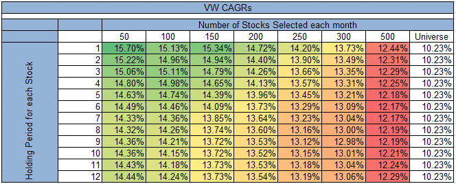
The results are hypothetical results and are NOT an indicator of future results and do NOT represent returns that any investor actually attained. Indexes are unmanaged, do not reflect management or trading fees, and one cannot invest directly in an index. Additional information regarding the construction of these results is available upon request.
The results below reflect the compound annual growth rates for the various strategies from 1970-2016 for equal-weighted portfolios. The monthly rebalanced 50 stock value strategy earns 17.01% CAGR, whereas the annually rebalanced 500 stock portfolio earns 13.97% CAGR. It is important to note that all of these results are GROSS of transaction costs.
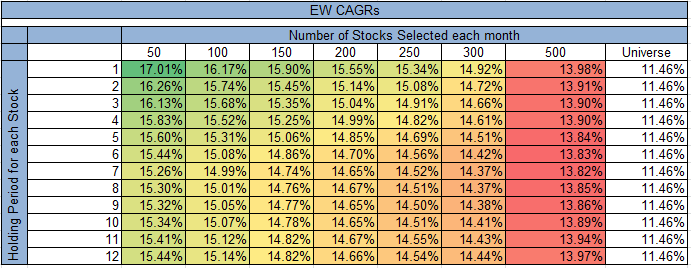
The results are hypothetical results and are NOT an indicator of future results and do NOT represent returns that any investor actually attained. Indexes are unmanaged, do not reflect management or trading fees, and one cannot invest directly in an index. Additional information regarding the construction of these results is available upon request.
There is a clear relationship between absolute returns and the number of firms, the holding period, and portfolio weightings. In general, it appears that 1) a more frequent rebalance, 2) a more concentrated portfolio, and 3) equal-weighting seem to increase returns and do so independently.
But not everything is perfect. We like to highlight one (potential) downside of a more concentrated portfolio — it will not track the value-weight index! One way to examine how the portfolios can vary from the passive index (in this case, the SP500) is to examine the tracking error of the portfolio relative to the SP500.(1)
Below we examine the tracking error of the value-weight portfolios relative to the SP500 from 1970 – 2016.
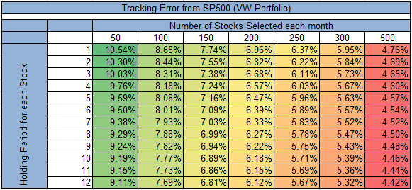
The results are hypothetical results and are NOT an indicator of future results and do NOT represent returns that any investor actually attained. Indexes are unmanaged, do not reflect management or trading fees, and one cannot invest directly in an index. Additional information regarding the construction of these results is available upon request.
Similarly, we examine the tracking error of the equal-weight portfolios relative to the SP500 from 1970 – 2016.
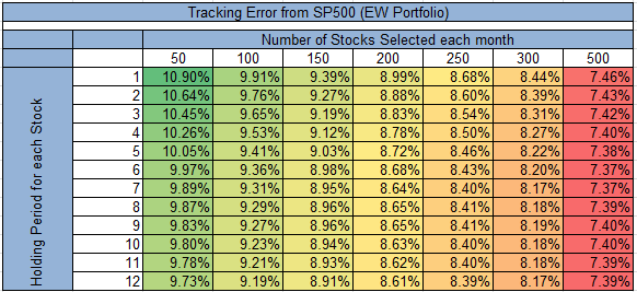
The results are hypothetical results and are NOT an indicator of future results and do NOT represent returns that any investor actually attained. Indexes are unmanaged, do not reflect management or trading fees, and one cannot invest directly in an index. Additional information regarding the construction of these results is available upon request.
What pops out of the results is the following — the more concentration (as well as more rebalancing), the higher the tracking error. We recommend any potential investor in a highly concentrated value portfolio understand this ahead of time and determine if one can withstand the tracking error pain.
Digging a little deeper into the results
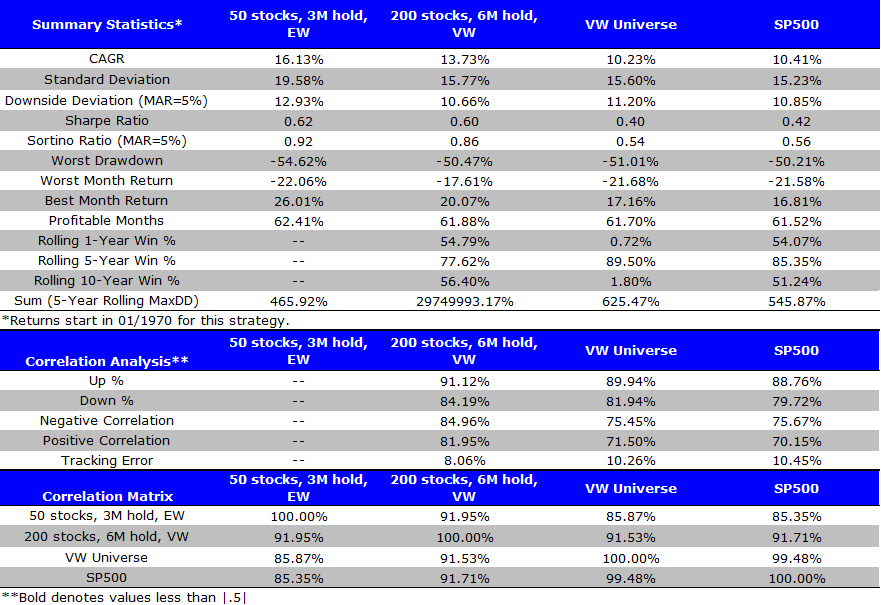
Let’s examine the returns (with some more advanced statistics) on two portfolios. First, we will examine the 50 stock, 3-month holding period portfolio (equal-weight), and compare this to a 200 stock, 3-month holding period portfolio (value-weight).
Here are the portfolios we examine:
- 50 stocks, 3M hold, EW = Top 50 firms ranked on EBIT/TEV, held in the portfolio for 3 months. The portfolio is equal-weighted.
- 200 stocks, 6M hold, VW = Top 200 firms ranked on EBIT/TEV, held in the portfolio for 3 months. The portfolio is value-weighted.
- VW Universe = Returns to the universe of our mid to large market capitalization firms (with available EBIT/TEV data). The portfolio is value-weighted.
- SP500 = S&P 500 Total return
Results are gross of management fees and transaction costs. All returns are total returns and include the reinvestment of distributions (e.g., dividends).
Here are the returns (1/1/1970-12/31/2016):
The results are hypothetical results and are NOT an indicator of future results and do NOT represent returns that any investor actually attained. Indexes are unmanaged, do not reflect management or trading fees, and one cannot invest directly in an index. Additional information regarding the construction of these results is available upon request.
Both equal weight and value weight value portfolios outperformed the index over the past 45 years (also note the high correlation between the universe of stocks and the SP500). The spread between the 50-stock and 200-stock portfolio is 2.40%–a number that will definitely make a difference over 45 years. There is also higher volatility associated with the value portfolios; however, as a component in a diversified portfolio structure, this risk differential is approximately zero. So the difference between the two value portfolios would primarily be the management fees (and perhaps higher frictional fees), the rebalance frequency (3 months versus 6 months), and the weighting (equal weight versus value weight) — more passive closet-index value portfolio will likely having a lower management fee than the equal weight, more concentrated and highly active value portfolio. The optimal long-term expected value portfolio will be determined by the spread in returns between the 1) expected benefits of the active constructed portfolio (~2.40% per year in the example above) and 2) the expected costs (e.g., management fees, frictional costs, etc). If the benefits are ~2.40% and the differential costs are 3.00%, we have a bad deal; if the benefits are 2.40% and the differential costs are 1% we may have a better deal.
Let’s get closer to the real world
Below is an example of two portfolio index constructions (data for the image below was derived on 4/19/2016).
- The x-axis represents “valuation” based on the percentile rank of EBIT/TEV across the universe of all stocks (1 = cheap, 0 = expensive).
- The y-axis represents “quality” based on the percentile rank of ROE across the universe of all stocks (1 = quality, 0 = junk).
- The dots reflect the percentage weight in the respective index.
- Blue = Quantitative Value Index (based of Wes’ book, Quantitative Value). <50 stock, equal-weight, quarterly rebalance
- Green = CRSP US Mid Cap Value Index (see methodology here). >200 stock, value-weight, quarterly rebalance
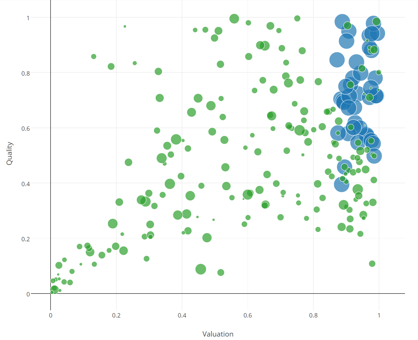
While the fundamental characteristics (cheapness, quality, etc.) of the portfolio holdings are much different depending on how the portfolio is constructed, this is often overlooked by investors. If one believes that firm characteristics, such as cheapness and quality, drive future expected returns, a portfolio construction that is more concentrated on those characteristics will do better than a portfolio that is less concentrated on these characteristics. Of course, these portfolios with more concentration on the characteristics desired will also have more tracking error (and typically more volatility) than a standard benchmark.
Learning Points
This simple discussion should highlight a few things:
- Value has historically worked on a gross of fee basis.
- Value works even better when it is concentrated and traded more frequently.
- Equal-weight portfolios work better than value-weight portfolios (even beyond size exposure)
- Investors should focus on portfolio construction and holdings characteristics when buying an investment fund.

About the Author: Jack Vogel, PhD
—
Important Disclosures
For informational and educational purposes only and should not be construed as specific investment, accounting, legal, or tax advice. Certain information is deemed to be reliable, but its accuracy and completeness cannot be guaranteed. Third party information may become outdated or otherwise superseded without notice. Neither the Securities and Exchange Commission (SEC) nor any other federal or state agency has approved, determined the accuracy, or confirmed the adequacy of this article.
The views and opinions expressed herein are those of the author and do not necessarily reflect the views of Alpha Architect, its affiliates or its employees. Our full disclosures are available here. Definitions of common statistics used in our analysis are available here (towards the bottom).
Join thousands of other readers and subscribe to our blog.