The blogosphere is spammed with commentary related to the current high market valuations and the inevitable crash that “must“ ensue.
We’ve even been involved in the conversation at different points, trying to add some depth to the broader debate. Our R&D lab has been cranking on various market indicators that go beyond “market expensive; therefore 50% drawdowns are around the corner” type analysis. In this post we discuss the usefulness of valuation spreads, or the spread between the average price for a bucket of cheap stocks and the average price for a bucket of expensive stocks.
Why valuation spreads might matter (maybe more than valuation levels)?
You’ve probably heard the statistics joke: your head is in the oven and your feet are in the fridge, on average you’re 72 degrees and life is great. Of course, you are also dead, and averages have managed to confuse us more than help us–a common flaw of statistical averages.
An analogous flaw of “averages” could be made in the context of financial markets. If the “average” P/E on the market is in the 99th percentile, people think the world is falling. Perhaps they’re right, but perhaps they need to dig a little deeper?
The problem with averages is they can’t communicate the “tails” of a distribution. Take 2 scenarios, each with an average P/E of 50:
- Scenario 1: 3 stocks in the universe: A, B, and C. PE_A=1, PE_B=50, and PE_C=99. The average P/E is 50, or in the 99th percentile of history.
- Scenario 2: 3 stocks in the universe: A, B, and C. PE_A=49, PE_B=50, and PE_C=51. The average P/E is 50, or in the 99th percentile of history.
By simply looking at average market valuations we miss some important information. As illustrated in the example above, averages don’t tell us much, on average (another statistics joke, sorry).
In scenario 1, there might be some amazing opportunity in the marketplace: stock A is selling at a PE of 1! With scenario 2, we might be more inclined to be afraid since all stocks are expensive. There are other scenarios one can draw up, which highlight the utter uselessness of averages. For example, imagine we witness a high market average PE of 35, but this PE is heavily skewed by a handful of mega-cap social media companies with PEs of 200+. What this high market average PE doesn’t tell us is that the other 95% of companies have a PE of 5!
An important disclaimer is in order: I am not claiming that average market PEs can’t be informative or useful, but I am making a broader point that one should consider other aspects of market valuations to get a clearer picture of what is actually going on in the marketplace. One example is normalized value spreads, or NVS…
How Do We Create Normalized Value Spreads (NVS)?
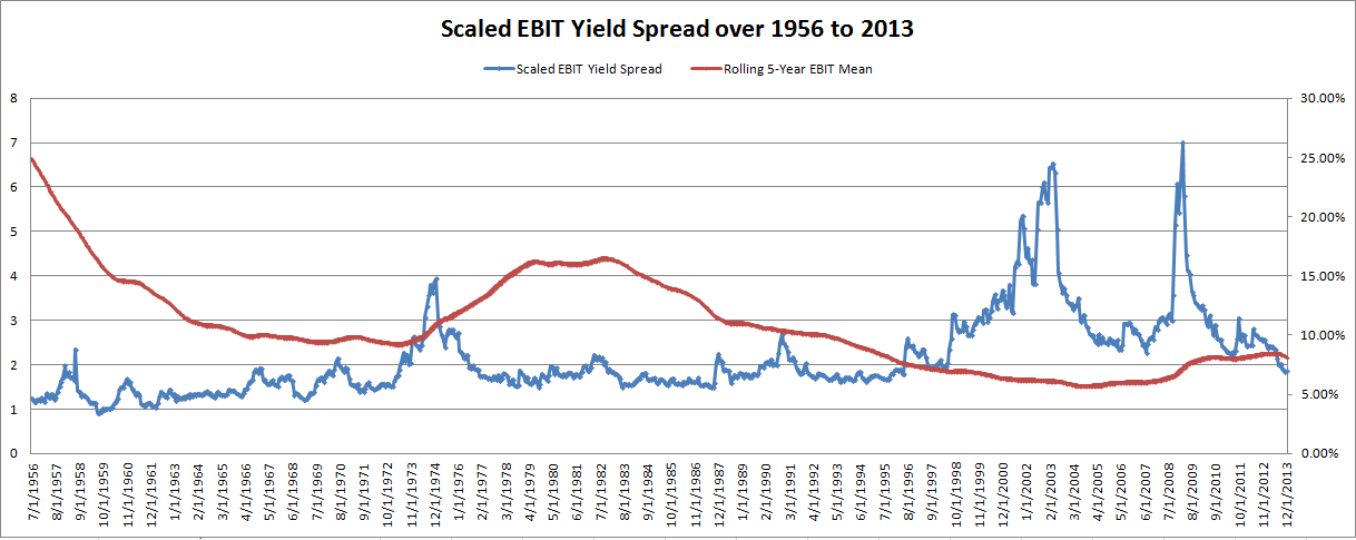
We take a look at the Scaled EBIT Yield Spread as our NVS from 7/1956 to 12/2013.
- Step 1: Sort stocks from the sample period into 10 deciles based on EBIT/TEV (we only focus on US mid/large cap to avoid weird micro/small cap outlier effects)
- Let’s say we have 1,000 stocks in the universe. We can calculate the EBIT/TEV for all stocks in the universe. We can then divvy the stocks into buckets–say, 10 deciles, or 100 stocks in each bucket.
- Step 2: Calculate the EBIT yield spread of each month= (average EBIT for the top 10% cheap) – (average EBIT for the bottom 10% expensive)
- Cheap EBIT/TEV decile has an average yield of 15%; expensive decile has an average yield of 5% ==> Value spread = 10%
- Step 3: Divide EBIT yield spread calculated in the previous step by its rolling 5-year EBIT yield mean. We get the Scaled EBIT Yield Spread over time.
- The rolling 5-year average EBIT yield for the universe is 10%. The Normalized Value Spread (NVS) = (15%-5%) / 10% = 1
What Does NVS look like over time?
Below we chart the 5-year rolling EBIT mean over time (right axis) and the normalized value spread (NVS) using EBIT/TEV (left axis).
The results are hypothetical results and are NOT an indicator of future results and do NOT represent returns that any investor actually attained. Indexes are unmanaged, do not reflect management or trading fees, and one cannot invest directly in an index. Additional information regarding the construction of these results is available upon request.
Point #1: 5-year rolling EBITs signal the market isn’t cheap–but we already knew that.
Point #2: NVS suggests that valuations are pretty tight. A tight NVS is common, but does break down through time. For example, NVS signaled huge spreads in the 1973-1975, 1998-2003, and 2008-2009 markets (i.e. large dislocations/volatility). These NVS spreads represent situations where the price on cheap stocks is much cheaper than the price on expensive stocks. Intuitively, this is a good time to hunt for value in the marketplace and might be a signal for “blood in the streets.”
Summary: We are in a high valuation, low valuation dispersion market.
Where do we take it from here?
NVS is a new concept we’ve been tossing around since the evidence is weak that valuations levels do much for tactical asset allocation. But perhaps there is an interaction between spreads and levels that enhances predictability? We’d love to hear about more research related to this concept. We’re cranking the numbers as well, but enjoy seeing independent analysis as a robustness test on our own work.
Some academic research says this is all bunk:
[Is the value spread a useful predictor of returns?] No. Two related variables, the book-to-market spread (the book-to-market of value stocks minus the book-to-market of growth stocks), and the market-to-book spread (the market-to-book of growth stocks minus the market-to-book of value stocks) predict returns but with opposite signs. The value spread mixes the cyclical variations of the book-to-market and market-to-book spreads, and appears much less useful in predicting returns. Our evidence casts doubt on Campbell and Vuolteenaho [2004. Bad beta, good beta. American Economic Review 94(5), 1249–1275] because their conclusion relies critically on using the value spread as a predictor of aggregate stock returns.

About the Author: Wesley Gray, PhD
—
Important Disclosures
For informational and educational purposes only and should not be construed as specific investment, accounting, legal, or tax advice. Certain information is deemed to be reliable, but its accuracy and completeness cannot be guaranteed. Third party information may become outdated or otherwise superseded without notice. Neither the Securities and Exchange Commission (SEC) nor any other federal or state agency has approved, determined the accuracy, or confirmed the adequacy of this article.
The views and opinions expressed herein are those of the author and do not necessarily reflect the views of Alpha Architect, its affiliates or its employees. Our full disclosures are available here. Definitions of common statistics used in our analysis are available here (towards the bottom).
Join thousands of other readers and subscribe to our blog.