We’ve had a few posts showing that asset allocation systems relying on market valuation indicators (e.g., Shiller CAPE ratios) as a timing signal may end up in disappointment…
- Can market Valuations Be Effective Market-Timing Signals?
- Dissecting Goldman’s 99 Percentile Market-Timing Signal
Nonetheless, we’ve continued on the quest to improve tactical asset allocation using market valuation data. The data speaks clearly when it comes to the association between valuations and long-term realized returns–high valuations are associated with low long-term realized returns. However, as Michael Kitces highlights, tactically allocating using valuation information is challenging. Moreover, there are arguments that the association between CAPE and LT returns may be more complex than previously thought.
In short, valuation-based asset allocation strategies haven’t been that exciting…but…
The folks at Gestaltu inspired us with a unique twist on basic valuation-based timing methodologies:
…we chose the cyclically adjusted earnings yield as the valuation metric, which is just the reciprocal of the Shiller PE. We then adjusted the yield value for the realized year-over-year inflation rate to find the real earnings yield. Finally, we used an ‘expanding window’ approach to find the percentile rank of the real earnings yield to eliminate as much lookahead bias as possible.
Note that because we are using real earnings yield rather than nominal earnings yield, markets can get cheap or expensive in three ways:
- changes in inflation
- changes in earnings
- changes in price
Gestaltu’s post used 1/CAPE as the valuation metric, or the “earnings yield,” as a baseline indicator; however, they “adjusted the yield value for the realized year-over-year (yoy) inflation rate,” by subtracting the year-over-year inflation rate from the rate of 1/CAPE.
To summarize, the metric looks as follows if the CAPE ratio is 20 and realized inflation (Inf) is 3%:
Real Yield Spread Metric = (1/20)-3% = 2%
Fairly simple.
Strategy Background:
We performed our own replication of the first two strategies from the post:
- Average Valuation based asset allocation: own S&P500 when valuation < long-term average, otherwise hold cash
- In other word, get out of the market if the real yield spread is below average.
- 80th Percentile Valuation based asset allocation: own S&P500 when valuation < 80th percentile, otherwise hold cash
- In other word, get out of the market if the real yield spread is extremely low.
Some adjustments are applied in the replication:
- Bureau of Labor Statistics (BLS) publishes the CPI on a monthly basis since 1913; however, the data is one-month lagged (possibly longer). For example, the CPI for January won’t be released until February. So when we subtract the year-over-year inflation rate from the rate of 1/CAPE, we do 1-month lag to avoid look-ahead bias.
- S&P Down Jones Indices publishes SP 500 index earnings on a quarterly basis and the data is one-quarter lagged. For example, the earnings for Q3 won’t be released until Q4. So we also take this into consideration to avoid look-ahead bias.
- We use the S&P 500 Total Return index as a buy-and-hold benchmark.
- Our back test period is from 1/1/1934 to 12/31/2014, while the article looks over the period from 1/1/1934 to 12/31/2012.
Results are gross of any fees. All returns are total returns and include the reinvestment of distributions (e.g., dividends). Indexes are unmanaged, do not reflect management or trading fees, and one cannot invest directly in an index.
Our Replication Results
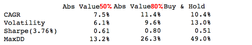
The first table shows the results from the Gestaltu post:
The results are hypothetical results and are NOT an indicator of future results and do NOT represent returns that any investor actually attained. Indexes are unmanaged, do not reflect management or trading fees, and one cannot invest directly in an index. Additional information regarding the construction of these results is available upon request.
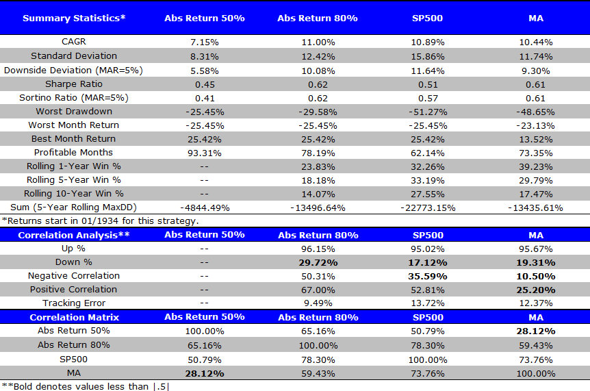
Our backtest results show similar CAGRs, but higher volatilities than the results from Gestaltu. This could be due to changes in experiment design. Overall, the “Abs Return 80%” strategy outperforms buy-and-hold while the “Abs Return 50%” strategy underperforms buy-and-hold. We include a long-term moving average rule for reference (S&P 500 if above 12-month MA, risk-free if below the 12-month MA).
Summary statistics are below:
The results are hypothetical results and are NOT an indicator of future results and do NOT represent returns that any investor actually attained. Indexes are unmanaged, do not reflect management or trading fees, and one cannot invest directly in an index. Additional information regarding the construction of these results is available upon request.
Bottom-line: The system looks promising.
Robustness Tests: Adjusting the Starting Point for the Look-Back Window
Gestaltu set 1/1/1924 as the starting date and then uses an expanding window as the look-back period.
We investigate how changing the start date affects results.
Results shown are from 1/1/1934 to 12/31/2014.
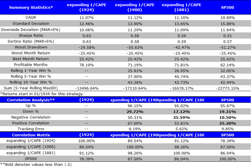
The table below shows the results of the “Abs Return 80%” strategy using different starting dates for the expanding window: 1924, 1900, and 1881. The starting date for the expanding window calculation can create marginal differences in the results. For example, the Sharpe ratios vary from 0.58 to 0.63. Overall, the results appear robust to the expanding look-back window start date.
The results are hypothetical results and are NOT an indicator of future results and do NOT represent returns that any investor actually attained. Indexes are unmanaged, do not reflect management or trading fees, and one cannot invest directly in an index. Additional information regarding the construction of these results is available upon request.
Bottom-line: The system looks promising.
Robustness Tests: Rolling Look-Back Window
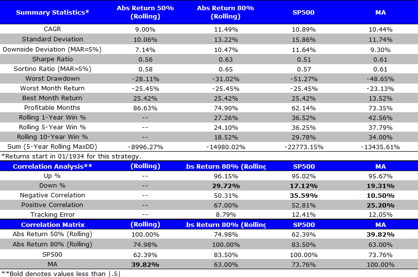
In this section we try a 10-year rolling look-back period calculation.
- For example, we measure the percent rank of CAPE on 12/31/2014 relative to the past 10 years (12/31/2004 to 12/31/2014); while an expanding window (results already shown above) would measure the percent rank of CAPE on 12/31/2014 relative to the whole time period (from the start date to 12/31/2014).
Results below highlight that a rolling-window technique yields similar results to the expanding-window technique.
The results are hypothetical results and are NOT an indicator of future results and do NOT represent returns that any investor actually attained. Indexes are unmanaged, do not reflect management or trading fees, and one cannot invest directly in an index. Additional information regarding the construction of these results is available upon request.
Bottom-line: The system looks promising.
Robustness Tests: Inflation-Adjusted PE Ratio
In this section, we use the old-fashioned price-to-earnings ratio in place of the CAPE ratio. We use a rolling 10-year window look-back method and adjust inflation with a 1-month lag.
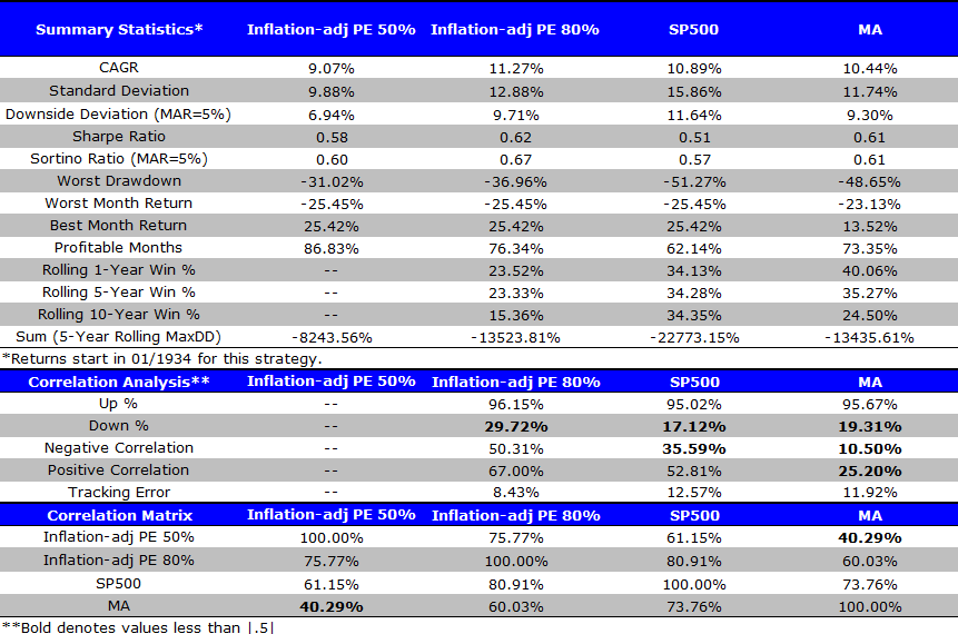
Full Sample Results: 1/1/1934 to 12/31/2014
- Inflation-adjusted PE strategies work better than buy-and-hold. They also work better than CAPE-based strategies.
The results are hypothetical results and are NOT an indicator of future results and do NOT represent returns that any investor actually attained. Indexes are unmanaged, do not reflect management or trading fees, and one cannot invest directly in an index. Additional information regarding the construction of these results is available upon request.
Bottom-line: The system looks promising.
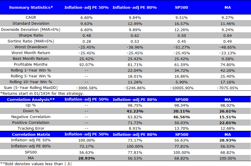
First Half Results: 1/1/1934 to 12/31/1974
- Inflation-adjusted PE strategies work OK in the first half.
The results are hypothetical results and are NOT an indicator of future results and do NOT represent returns that any investor actually attained. Indexes are unmanaged, do not reflect management or trading fees, and one cannot invest directly in an index. Additional information regarding the construction of these results is available upon request.
Bottom-line: The system looks promising.
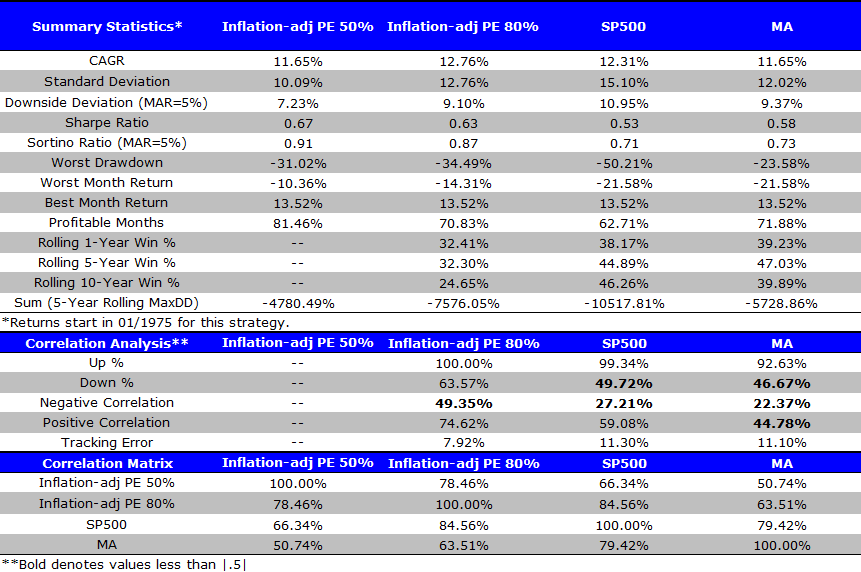
Second Half: 1/1/1975 to 12/31/2014
- Inflation-adjusted PE strategies work well in the second half.
The results are hypothetical results and are NOT an indicator of future results and do NOT represent returns that any investor actually attained. Indexes are unmanaged, do not reflect management or trading fees, and one cannot invest directly in an index. Additional information regarding the construction of these results is available upon request.
Bottom-line: The system looks promising.
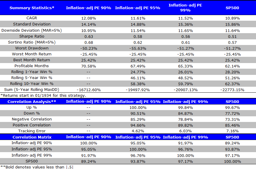
Robustness Tests: Different Thresholds
In this section we look at different percentile thresholds to determine the timing signal. For example, the results are strong when the timing signal is based on the average or the 80th percentile, but what happens if we use different signals? We use a rolling 10-year window look-back method and adjust inflation with a 1-month lag.
Full Sample: 1/1/1934 to 12/31/2014
- Higher thresholds increase maximum drawdowns (relative to lower thresholds, such as the 50th and 80th percentiles). The results are better than pure buy-and-hold, but this does highlight a potential robustness issue.
The results are hypothetical results and are NOT an indicator of future results and do NOT represent returns that any investor actually attained. Indexes are unmanaged, do not reflect management or trading fees, and one cannot invest directly in an index. Additional information regarding the construction of these results is available upon request.
Bottom-line: The system may have robustness issues.
Robustness Tests: Staggered Allocations
In this robustness test, we vary holding percentages based on the percentile rank of earnings_yield – realized inflation. For example, if last month’s E/P – CPI is in the 12th percentile based on the past , then we allocate 12% to stock and 88% to T-bills. We use a rolling 10-year window look-back method and adjust inflation with a 1-month lag.
Full Sample: 1/1/1934 to 12/31/2014
- Staggered allocations strategies are better than buy-and-hold
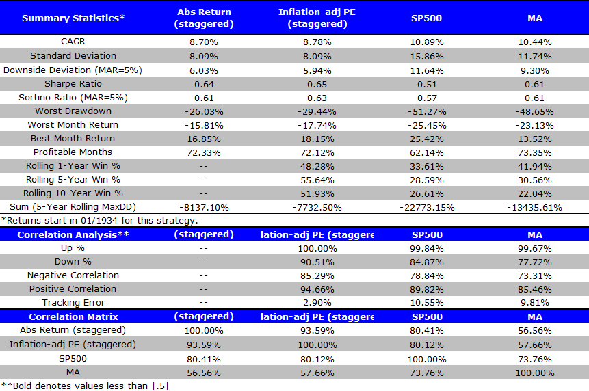
The results are hypothetical results and are NOT an indicator of future results and do NOT represent returns that any investor actually attained. Indexes are unmanaged, do not reflect management or trading fees, and one cannot invest directly in an index. Additional information regarding the construction of these results is available upon request.
Bottom-line: The system looks promising.
Robustness Tests: Changing the Real Inflation Component of the Signal
In the post, “Market Valuations based on CAPE – A Deeper Dive“, we take the 1/CAPE and subtract the inflation adjusted 10-year U.S. Treasury yield, so that we can examine how expensive the market is relative to real returns available via a bond alternative (a stock investor would prefer a higher spread, all else being equal).
To summarize, the metric looks as follows if the CAPE ratio is 20, realized inflation (Inf) is 3%, and the 10-Year Treasury is 5%:
Real 10-Year Spread Metric = (1/20)-(5-3)% ~ 3%
Full Sample: 1/1/1934 to 12/31/2014
- This new measure doesn’t work–at all.
- Understanding why a seemingly small change in technique destroys the results is puzzling and worthy of more investigation…
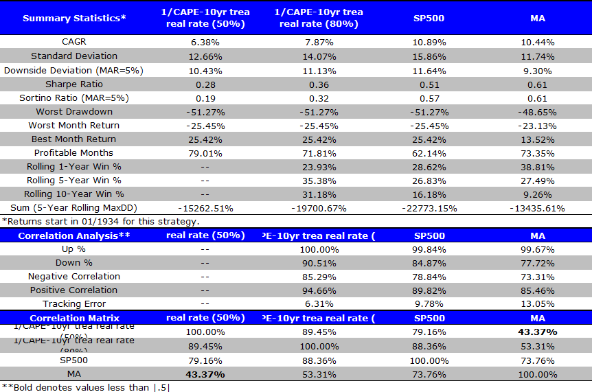
The results are hypothetical results and are NOT an indicator of future results and do NOT represent returns that any investor actually attained. Indexes are unmanaged, do not reflect management or trading fees, and one cannot invest directly in an index. Additional information regarding the construction of these results is available upon request.
Bottom-line: The system may have robustness issues.
Conclusion
After enduring years of frustration trying to identify a valuation-based asset allocation technique–that actually worked–I think the team at Gestaltu is on to an interesting concept. By simply looking at real spreads between equity valuations and realized inflation (high spreads are good for equity; low spreads are bad for equity), one can devise a timing rule that captures most of the upside, but protects on the downside. Of course, this is all historical data and could very well be an exercise in data-mining. That said, the concept of buying equity assets when they have much higher yields than current inflation, is intuitively appealing.
We’ll continue our investigations into the subject, but we wanted to give a quick view into some of our high level research on the subject.

About the Author: Wesley Gray, PhD
—
Important Disclosures
For informational and educational purposes only and should not be construed as specific investment, accounting, legal, or tax advice. Certain information is deemed to be reliable, but its accuracy and completeness cannot be guaranteed. Third party information may become outdated or otherwise superseded without notice. Neither the Securities and Exchange Commission (SEC) nor any other federal or state agency has approved, determined the accuracy, or confirmed the adequacy of this article.
The views and opinions expressed herein are those of the author and do not necessarily reflect the views of Alpha Architect, its affiliates or its employees. Our full disclosures are available here. Definitions of common statistics used in our analysis are available here (towards the bottom).
Join thousands of other readers and subscribe to our blog.