Want to Learn Way Too Much About Stock Market Factors? Read This Paper.

During the past few decades, newly discovered stock anomalies have been embarrassing existing factor models, such as the Fama-French 3-factor.

As many readers know, each long or short “leg” of these popular long/short factor portfolios is generally constructed by ranking stocks on one specific characteristic (value, momentum, or volatility).

For example, take the Fama French 3-factor model. First, it relies on HML (the value factor), which is the excess returns of value stocks over growth stocks (size-adjusted). Second, it uses SMB (the size factor), which is simply the excess return of small caps over large caps (value-adjusted). The third factor is market risk, or “beta.” Observed excess returns (i.e., returns above and beyond the risk-free rate) can often be explained when one controls for these factor characteristics.

However, none of these single mispricing factors (i.e. HML, SMB, MOM) can accommodate a large set of anomalies very well. When you look at a larger set of anomalies, such as 30 or 50 or more anomalies, models such as the Fama French 3-factor model, do not have a strong ability to explain the larger number of anomalies analyzed. Of course, this may not be too surprising since anomalies are typically only deemed “anomolous” once it is determined that the FF 3-factor model can’t explain the excess returns associated with the strategy that generates the anomaly.

Stambaugh and Yuan (2015) say they can solve this problem by constructing two composite factors, each of which is made up of clusters of anomalies that are similar to and better represent the single-characteristic factors in the parsimonious models.
Thus the key difference is:

“Rather than have each factor correspond to a single anomaly, as is typical, we construct factors by combining stocks’ rankings with respect to 11 prominent anomalies.” 

** These 11 prominent anomalies are: net stock issues, composite equity issues, accruals, net operating assets, asset growth, investment to assets, distress, O-score, momentum, gross profitability, and return on assets.

Next, the authors combine these two new factors with market and size factors, in order to create a new four-factor model. This model is demonstrated to perform better than notable four- and five-factor alternative models.

From the paper:

For example, when applied to the 51 of those anomalies having data over our entire sample period, the Gibbons-Ross-Shanken (1989) test of whether all the anomalies’ alphas equal zero produces a p-value of 0.10 for our model compared to 0.003 or less for these four- and five-factor alternative models.

Note that a Gibbons-Ross-Shanken test has as a null hypothesis that there is no alpha associated with these anomalies. So if you find alpha, the model is not doing a good job.

Mispricing factors: UMO (underpriced minus overpriced)

It is a complex process to construct the mispricing factors. Below we simplify some key steps:

• Step 1: Separate the 11 anomalies into two clusters using a correlation-based distance measurement and a clustering method.
• Step 2: Average a stock’s rankings with anomaly measures within each of the two clusters. Thus, each month, a stock has two composite mispricing measures, P1 and P2.
• Step 3: Construct a UMO1 (underpriced minus overpriced) factor: the paper describes UMO1 as “value-weighted returns on each of the four portfolios formed by the intersection of the two size categories with the top and bottom categories for P1. UMO2, is similarly constructed from the low- and high-P2 portfolios.”

Then the paper combines the two mispricing factors with market and size factors to produce a four-factor model. (This paper also constructs its own size factor rather than use the FF size factor. Check it out if you are interested).

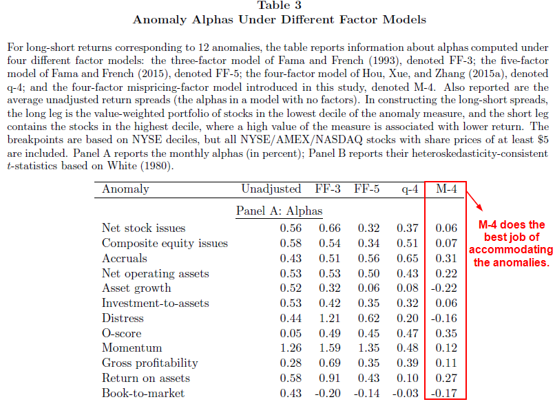
The authors then run a horse-race comparison among four factor models:

• FF-3: three-factor model of Fama and French (1993)
• FF-5: five-factor model of Fama and French (2015)
• q-4: four-factor “q-factor” model of Hou, Xue, and Zhang (2015a)
• M-4: four-factor mispricing-factor model introduced in this paper

The results from table 3 demonstrate that the M-4 model performs better and accommodates a wider range of anomalies than both FF-5 and q-4 models. Specifically, eight out of the nine positive M-4 alphas are lower than any of the corresponding alphas for the other models.

Also, if we replace the two mispricing factors with a single composite mispricing factor that simply averages rankings across the entire 11 anomalies, the subsequent 3-factor model outperforms the FF-3.

The results are hypothetical results and are NOT an indicator of future results and do NOT represent returns that any investor actually attained. Indexes are unmanaged, do not reflect management or trading fees, and one cannot invest directly in an index. Additional information regarding the construction of these results is available upon request.

Perhaps this isn’t surprising, since the factor model used to “control” for the anomalies is built using the anomalies (the same critique can be said for the other factor models–e.g., value washes away when you control for HML). However, the authors do examine a larger set of 73 anomalies and show that their factor model works better than other factor models. Pretty cool.

At a minimum, for researchers looking to identify “new” ideas, this factor model is a great tool. If one identifies a significant “alpha” after controlling for the Stambaugh and Yuan 4 factor model, there is a good chance there may be something special associated with the strategy under review. Finally, this is a 93-page monster on everything “factor” related. If you felt like geeking out over the weekend, this is a good place to start!

Mispricing Factors

• Stambaugh and Yuan
• A version of the paper can be found here.
• Want a summary of academic papers with alpha? Check out our Academic Research Recap Category.

Abstract:

A four-factor model with two “mispricing” factors, in addition to market and size factors, accommodates a large set of anomalies better than notable four- and five-factor alternative models. Moreover, our size factor reveals a small-firm premium nearly twice usual estimates. The mispricing factors aggregate information across 11 prominent anomalies by averaging rankings within two clusters exhibiting the greatest co-movement in long-short returns. Investor sentiment predicts the mispricing factors, especially their short legs, consistent with a mispricing interpretation and the asymmetry in ease of buying versus shorting. Replacing book-to-market with a single composite mispricing factor produces a better-performing three-factor model.