Commodity Futures Investing: Complex and Unique

Commodity futures investing is arguably the most misunderstood asset class in the financial marketplace.

We want to change that state of affairs.

Commodity futures strategies are fascinating and can be beneficial to investors. However, commodity futures are often complex, involve leverage and significant volatility, and have suffered periods of poor performance for decade-long periods (the last 10 years is a good example).

Nonetheless, because of the unique properties of the asset class, sophisticated investors should at least consider commodity futures as part of their investment toolkit, and at the very least, consider the exploration into commodity futures as part of a dedication to education and becoming a better investor.

We begin our exploration with two simple questions that investors should consider regarding all investments:

1. What are they buying?
2. Why are they buying it?

This post helps investors check both of those boxes if they choose to invest in commodity futures-based investment strategies.⁽¹⁾

A PDF version of this is available here.

An Introduction to Commodity Futures

Commodity futures investing can appear to be deceptively simple, and investors can have basic misunderstandings about the asset class. For example, many investors (including the great investors at GMO) hint at the idea that investing in commodity-producing equities is “better” than investing in the underlying commodity futures. If this were true it would be great on many levels — more transparent, more liquid, more tax-efficient, and less complex. But there is a problem — one can’t replicate commodity future trading strategies via equities because there are 2 elements of commodity futures: spot returns and roll yield return. Commodity equities and commodity futures are different animals that help investors often achieve different goals. ⁽²⁾

We’ve written about commodity exposure and commodity investing. And while commodity equities and commodity futures can be similar, there are profound differences when one digs into the weeds. What commodity futures can provide for a diversified portfolio is also very different from what commodity equities provide for a diversified portfolio (i.e., more equity risk).

In many respects, commodity futures offer variations of commodity-related exposure, offerings premiums that are only loosely or partially related to commodity prices themselves. For example, we posted here about commodity strategies when discussing a Fuertes et al. paper that describes a strategy that combines momentum and term structure (e.g., roll yield) signals.

There have been a number of papers over the past decade that have explored commodity futures returns from different perspectives. By examining the literature, some competing views emerge, but collectively they contribute to a better understanding of the asset class.

Back in 2006, Gorton and Rouwenhorst (GR) wrote a seminal paper about futures that showed that an equally-weighted index of commodity futures from 1959 to 2004 had equity-like returns, performed better in periods of unexpected inflation, and had a negative correlation with traditional asset classes. In short, there seemed to be a lot to like about the asset class, especially as a diversifier.

From the paper:

Fully-collateralized commodity futures have historically offered the same return and Sharpe ratio as equities. While the risk premium on commodity futures is essentially the same as equities, commodity futures returns are negatively correlated with equity returns and bond returns.

Similar performance, but with a negative correlation to equity and bonds? This is an asset allocator’s dream come true!

Backtests Work…Until they Don’t!

Of course, for the decade following the results from the GR paper, some researchers identified that the returns to commodity futures stunk it up.

For example, Erb and Harvey (2015) observe that long-only commodity returns for the Bloomberg Commodity Index and the S&P GSCI commodity index over the period were -4.6% per year, which was a much lower return than for stocks and bonds. The chart below highlights the poor performance over the most recent decade. Yuck!

Graph from Erb and Harvey Highlighting Poor BCOM/GSCI Commodity Index Returns

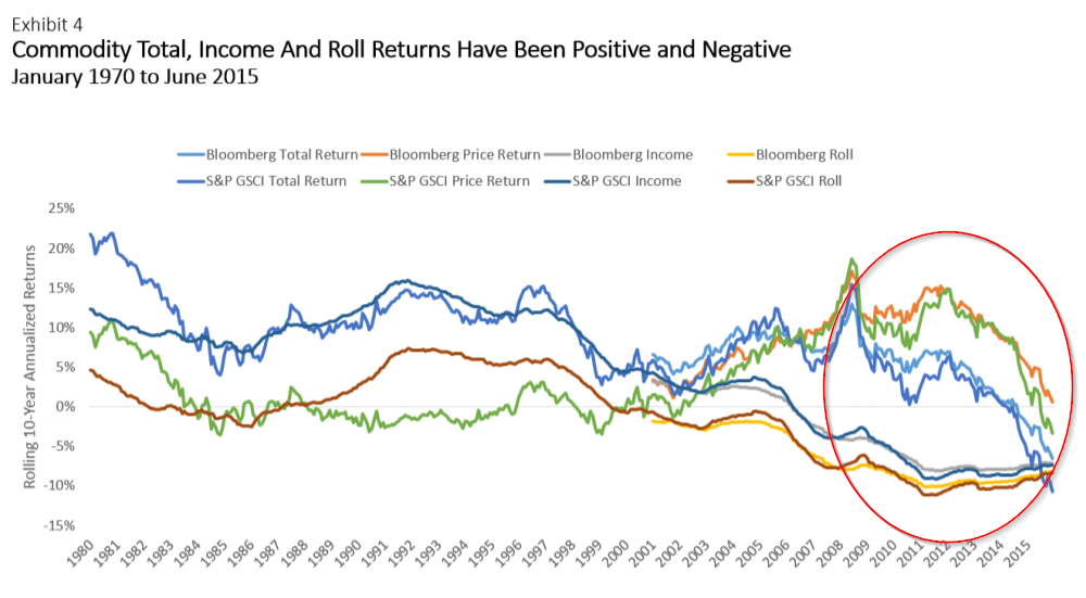
Erb and Harvey note that a key driver of these returns was a poor “income return” over the recent period (roll yield plus collateral return). Erb and Harvey leverage this fact to make the reasonable argument that investors expecting to earn a “safe” carry return from investing in commodity futures may be disappointed. Periods of poor income returns from commodity investments are certainly possible and can be expected to last for fairly long (10 years) time frames. In short, commodity futures investing is definitely risky!

Wait…Maybe the Backtests Were Correct?

Erb and Harvey paint a picture that perhaps investors should question the historical performance of commodity futures. Perhaps the historical returns were an artifact of data-mining and/or a lucky streak in commodities during the original GR paper time period?

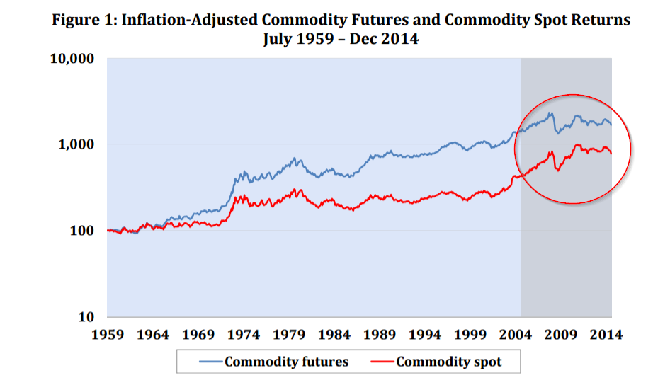
To combat the arguments in Erb and Harvey (2015), Bhardwaj, Gorton, and Rouwenhorst wrote a 2015 paper that found that 10-years of additional data (2005-2014) did not change their basic conclusions from Gorton and Rouwenhorst (2006): The average risk premium to an equal weight commodity futures index during this out-of-sample period was 3.7% per annum, which is comparable to its long-term in-sample average of 5.23% from 1959-2004. The authors attributed much of the lower out-of-sample returns to lower collateral returns. The chart below highlights their core result that commodity futures haven’t been wonderful in the past decade, but they haven’t been a tragedy either:

Graph from Bhardwaj, Gorton, and Rouwenhorst Highlighting Equal-Weight Commodity Index Returns

Two Research Groups with Two Different Conclusions: What gives?

Erb and Harvey find that commodities “don’t work” post GR, whereas, Bhardwaj, Gorton, and Rouwenhorst (2015) highlight that the performance of commodity futures is arguably consistent with their historical estimates.

Why are the conclusions so different? The different results are driven by different methodologies.

In the Erb and Harvey paper, the authors look at indices that are weighted by trading volume or macroeconomic factors. Indirectly, this portfolio construction skews the results to overweight the experience of energy futures (oil in particular).⁽³⁾

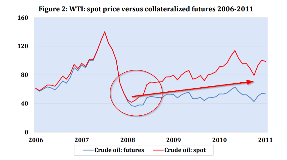
Heavy exposure to energy futures would also explain why Erb and Harvey calculate such a large negative “roll yield” estimate relative to the results in Bhardwaj, Gorton, and Rouwenhorst. Oil futures structurally moved to a strong “contango” state, following the 2008 crisis. The intense negative roll yield prevented oil futures from capturing the gains in the spot returns (red line in the chart below versus the blue line).⁽⁴⁾

In contrast, Bhardwaj, Gorton, and Rouwenhorst look at equal-weighted commodity futures indices, which minimize the influence of a single commodity contract, and are arguably a better reflection of a commodity future investment strategy an investor would actually utilize in practice. ⁽⁵⁾

Amazingly, a seemingly small difference in construction (equal-weight vs. volume/macro weight) leads to incredibly different out-of-sample results.

But both sets of authors agree on a simple truth: investors need to know what they are buying.

The authors also all agree that commodity future returns are driven by 2 components: spot return and roll yield.

Great. We’re in agreement. But let’s dig a bit deeper.

Understanding Commodity Futures Returns

Just when we thought Erb and Harvey, and the Bhardwaj, Gorton, and Rouwenhorst team had a corner on the commodities market (yes, this is an attempt at a bad joke), the crew at AQR (and NYU) came out with a paper on commodity futures.⁽⁶⁾ We will use this paper as an anchor for understanding commodities because it serves as the most comprehensive study on the subject and benefits from being able to stand on the shoulders of prior research.

The key differentiation of “Commodities for the Long Run” from prior research is the use of an unusually long data set that begins in 1877. The authors find that the long-run commodity future return premia are robust, perform well during inflation, and have the potential to serve as a great diversifier in a stock/bond portfolio. In the authors’ words:

…commodity futures can add value to a diversified portfolio from an asset allocation perspective.

But before we dig into the details of the paper, we will cover some basics of commodity futures investing.

The Mechanics of Commodity Futures Pricing

In order to grasp where roll returns, or “roll yield,” come from, we must first understand how futures are priced in equilibrium.

Futures price reflects three components set forth in the equation below (outlined in detail below):⁽⁷⁾

F = Sp*(1+r+s-c)

The components of the equation are as follows:

1. The Risk-free rate, r, is embedded in the futures price due to the leverage inherent in commodity futures.
2. Storage costs, s, are the annualized costs to store a physical commodity. 
3. Convenience yield, c, arises from the benefit of holding a physical commodity.
4. Sp is the current spot price.
5. F is the current future price.

Question: Where did this magical equation come from?

Answer: arbitrage.

Consider that an investor always has two options to pursue if they want to own a specific commodity at time T:

1. Borrow money, buy the commodity, store it, and hold it until time T.
2. Go long the future and settle the future at time T.

Let’s put some numbers out there to make this more tangible.

Goal: We want to own a  gold bar a year from now.

Assumptions:

• Sp = Gold bars trade at $1000 (i.e., spot rate)
• r = Interest rates are 5%
• s = Storage costs are 3% a year (e.g., buying a safe, a gun, etc.)
• c = Convenience yield are 10% a year (e.g., there is a high chance of a government meltdown and owning physical is beneficial)
• F = 1 year futures on a gold bar are $1000

Strategy #1, the “borrow and bury” approach, will work as follows:

• Borrow $1000 and buy a gold bar. In one year this will cost $1000*(1+5%) = $1050.
• Pay $30 (3%) to bury the gold bar in a safe in your backyard.
• Gain $100 in convenience benefits because you’ll have gold if/when the world blows up.
• Strategy #1 payoff = Sp_T – $1050 -$30 + $100, where SpT is the future value of a gold bar (which we don’t know today)

Strategy #2, the “buy futures” approach, will work as follows:

• Go long a 1-year gold bar futures contract at $1000. We now have the obligation to pay $1000 in one year for a gold bar, which will be worth Sp_T.
• Strategy #2 payoff = Sp_T – $1000

Both of these strategies achieve our goal: own a gold bar a year from now. And because both strategies deliver the same thing, their payoffs should be the same.

Let’s see how the math plays out:

• Strategy #1 payoff (borrow and own) = Sp_T – $1050 -$30 + $100 = Sp_T – $980
• Strategy #2 payoff (enter futures contract @ $1000) = Sp_T – $1000

So based on current prices in our example, if you want to own a gold bar a year from now, you’d rather borrow, own, and bury a gold bar in your backyard, than enter into a futures contract. Both strategies deliver a gold bar, but strategy #1 does it for $20 less!

Strategy #1 is dominant because Strategy #2 is too expensive. But what happens when the price of something is too high? Prices fall!

Arbitragers will take advantage of this opportunity by selling short futures and borrowing money and owning spot (i.e. buying gold bars). This profitable activity will end when the futures price (F) reaches approximately $980. When F = $980, the payoff to both strategies is equalized:

• Strategy #1 payoff (borrow and own) = Sp_T – $1050 -$30 + $100 = Sp_T – $980
• Strategy #2 payoff (enter futures contract @ $1000) = Sp_T – $980

Note that strategy #1 and strategy #2 now have equal payoffs, driven by marketplace arbitrage. Mathematically, one can sort this all out via equations:

First, in order to eliminate arbitrage, the payoffs for strategy #1 and strategy #2 must be equal:

Sp_T – Sp(1+r)+Sp*s-Sp*c = Sp_T – F,

which can also be written as follows,

Sp_T – Sp(1+r+s-c) = Sp_T – F,

and be rearranged to solve for F, the futures price:

F = Sp(1+r+s-c)

Plugging in our numbers to equation #3,

F = $980 = $1000*(1+5%+3%-10%)

In short, the futures price is equal to the spot price, adjusted for the cost of borrowing, the cost of storage, and taking into account the benefit of ownership (convenience yield).⁽⁸⁾

There you have it. If interest rates and storage costs are higher than convenience yields, futures have higher prices than spot (i.e., contango). If interest rates and storage costs are lower than convenience yields, futures prices are lower than spot (i.e. backwardation). Futures are essentially ownership of an asset in the future, secured by a loan, and the costs/benefits of ownership during the loan period are endured by another party.

Futures pricing 101.

Roll Yield and Futures Pricing

As time passes, a futures contract will converge on the spot price as the time period between the future’s expiration date and the current date converge on the same value.

What does this imply about the futures curve, assuming spot prices don’t change?

Well, if futures are above spot (contango), we can expect to earn negative returns as time passes and the future’s price converges on the spot price. Similarly, if futures are below spot (backwardation), we can expect them to creep up towards the spot price as time passes. This element of return that isn’t explicitly tied to the spot price is often referred to as “roll yield,” or the roll returns.

Let’s take a simple example to see how futures returns can be decomposed into spot and roll returns (we are going to ignore borrowing/lending and other details for now in order to demonstrate the spot/roll concept first).

It is January 2016, and the spot price of crude oil is $55. We go long the March futures contract at $50. Note that the futures curve is in “backwardation,” and slopes downward.

Now let’s say it’s February 2016, and we close our March contract at $60. What are returns for futures, decomposed into spot and roll returns?

• The futures return is: $60/$50-1 = 20%
• The spot return is: $60/55-1 = 9%
• The roll return is 11%, which is the difference between the futures and the spot returns (20%-9%=11%)

Using this approach, we can calculate spot returns, and derive roll returns for any rolled price series.⁽⁹⁾

Digging into Commodities for the Long Run

At the outset we mentioned that investors should always understand two elements when making an investment decision:

1. What they are buying.
2. Why they are buying it.

Hopefully, the prior section helped investors understand what they are buying when it comes to commodity futures — an element of spot price movements and elements of roll yield.

Now that we understand what we are buying we can try to understand why we would want to buy it. In other words, What are the expected returns? How do commodity futures work in different environments? What are the correlations with other asset classes? and so forth.⁽¹⁰⁾

Commodity Futures Expected Returns

“Commodities for the Long Run” looks at the performance of commodity futures over a long sample running from 1877 to 2015. 1877 was chosen as the starting point, since that was when records associated with early commodity futures contracts are first available, including data on corn, wheat, oats, lard, short ribs and pork. Over time additional commodities were added, including cotton soybeans, soymeal, soyoil, and others. The most recent data includes commodity data from across the complex.

The table below shows the arithmetic mean and volatility of each futures return, with returns broken down into the two components from above:

1. Excess Spot Return (spot return – risk-free rate): Going back to our pricing section, this component represents the fact a long futures is ownership of spot in the future, secured by a loan that must pay interest.
2. Interest Rate Adjusted Carry (convenience yield – storage costs): This aspect of futures represents the benefits/costs of owning physical and is indirectly paid to the long futures buyer. ⁽¹¹⁾

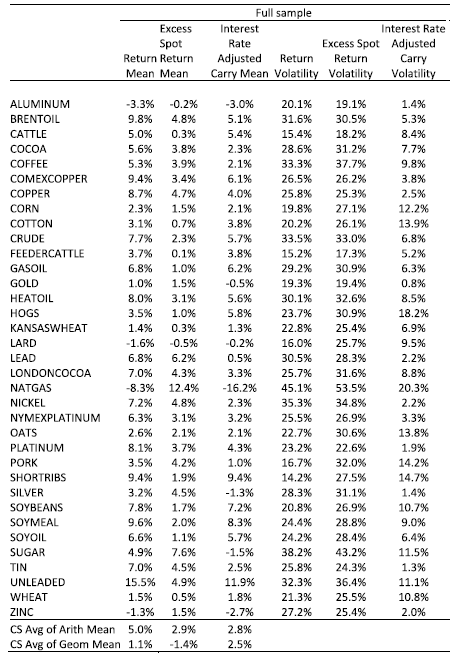
The series shows predominantly positive mean returns, both for excess spot and for interest rate adjusted carry. Also, 21 of the 35 commodities in the sample have higher interest rate adjusted carry than excess spot returns. So while spot returns make up a good part of futures returns (at least for arithmetic returns), certainly convenience yields are also a very important part of returns. Another thing that really stands out is the huge variability of spot returns, as compared with interest rate adjusted carry returns. Clearly, spot returns drive the variability in futures returns, rather than interest rate adjusted carry yields.

Visualizing Commodity Future Expected Returns

In order to assess what happens in a commodity future portfolio, the authors form two separate long-only portfolios, rebalanced monthly:

1. Equally-weighted portfolio of available commodity futures
2. Risk-weighted portfolio, with weights based on the contribution of each commodity to portfolio variance

Results for the two portfolios are similar, so we will mostly report results for equal-weights (see the paper for risk-weight results).

The graphs below plot the equal-weight cumulative commodity index returns for the period 1877-2015 based on the following:

• Left: i) spot – risk-free rate, and ii) interest-rate adjusted carry (convenience yield – storage costs)
• Right: i) spot returns and ii) roll yield (convenience yield – storage costs – risk-free rate):

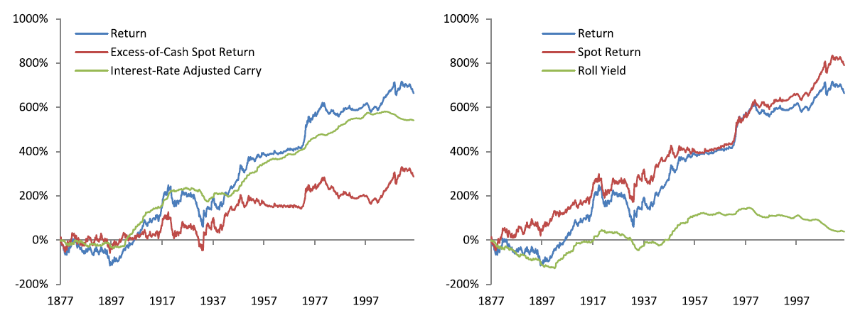
Overall, the blue line, which represents the excess return on commodity futures, points in the right direction. There is a time dilation effect, however. While the invested growth charts “looks good,” the time scale hides the painful reality that there are many periods of mediocre returns over long stretches of time.

While the left and right graphs are mathematically equivalent, note how the allocation of the continuously compounded (short-term) rate matters for return attribution. Practitioners often report the carry, or roll yield, of the commodity in spot/roll terms as depicted by the right graph. In this decomposition, carry on a standalone basis has earned approximately zero over the past 139 years (note: we discuss a more granular decomposition in the following section).

Intuitively, the left graph may be a more appropriate perspective. As was mentioned in the prior sections, a long future position can be broken into two pieces: 1) ownership of spot in the future, secured by a loan that must pay interest (spot – interest costs) and 2) net convenience yield (i.e., interest rate adjusted carry). In this view, interest rate adjusted carry is the natural premium that producers and buyers of commodities are willing to pay to speculators in order to avoid supply disruption in their business. After considering this interest rate adjusted carry, all that remains in the futures return is the spot price (which is unrelated to convenience) less cash returns. And if the futures were fully collateralized, the interest costs would approximately net out, under the assumption haircuts were minimal. ⁽¹²⁾

Expected Returns Across Regimes

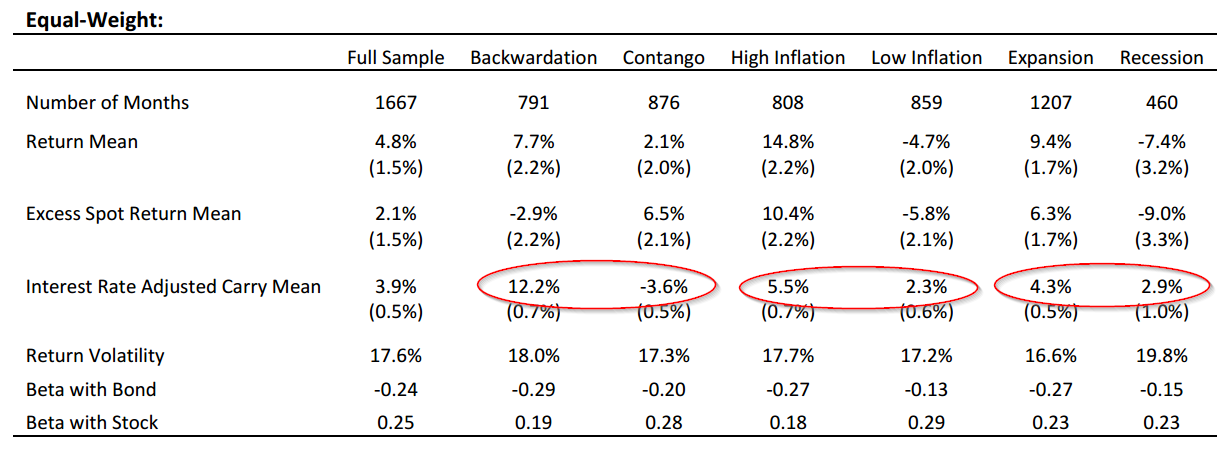
The invested growth figures highlight the attribution analysis of generic commodity futures strategies, independent of the market environment. The chart below documents the behavior of interest rate adjusted carry and excess spot returns over several markets, inflation, and term structure regimes.

The authors identify some core findings:

• Markets were fairly equally divided between backwardation and contango.
• During periods of backwardation, expected returns for long-only commodity futures were much higher and likely driven by interest rate adjusted carry.
• High inflation regimes were also positive for commodity future returns. These returns are driven by a mix of spot returns and interest rate adjusted carry.

The analysis above is interesting, but as the authors point out, it is likely the case that variables are correlated across these states. For instance, inflationary effects are correlated with returns during these expansions/contractions, which may imply a spurious correlation for futures returns during expansions/contractions.

Examining Returns via a Multivariate Analysis

The authors attack this issue via multivariate analysis by isolating carry, inflation, and business cycle as coefficients in regression. The output is below:

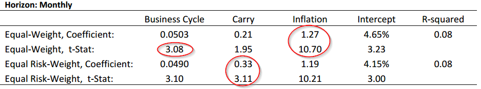
The results appear consistent with the prior chart. Coefficients for carry, inflation, and business cycle are all positive and statistically significant. The inflation coefficient is 1.27, which implies a nearly direct relationship with inflation, and with a very high t-statistic of 10.7. The business cycle (measured via a binary term) has statistically significant predictive power. Carry also explains returns: in particular, risk-weighted carry has a 0.33 coefficient, with a strong t-statistic of 3.11. Thus, carry seems to explain a reasonable portion of index returns here too. Interesting.

Commodity Future Returns versus Other Assets Across Regimes

Up until this point the discussion regarding commodity future return analysis has been independent of other investment alternatives. In the table below the authors report the mean, volatility, and Sharpe ratios for classic asset classes (we assume these are nominal returns, but it is unclear based on the text), as well as for different asset allocation methodologies that allocate across stocks, bonds, and commodities:

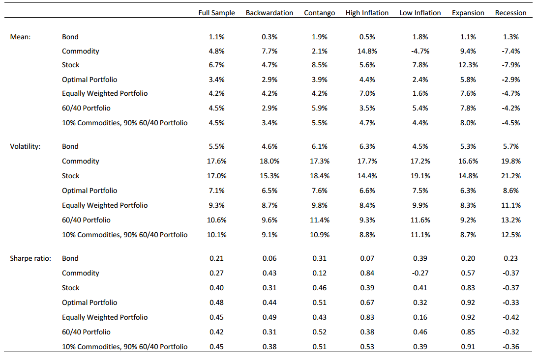
Once again, we can see how commodity futures contribute to returns during inflationary periods, and backwardation states, which contributes to the intuition of their value as a diversifier. It’s also interesting that the equally-weighted portfolio has a Sharpe ratio of 0.45 which is very close to the mean-variance optimized portfolio of 0.48. Despite all that heavy optimization work, risk-adjusted returns are still pretty similar to an equal-weight allocation. We have discussed aspects of equal weight allocations previously, in papers about tactical asset allocation and asset allocation.

Can Commodity Futures Enhance a Portfolio? Yes

The table above highlighted the unique benefits of commodity futures relative to other asset classes. Commodity futures do well in inflationary periods. Additionally, they outperform during backwardation states, which provides idiosyncratic returns compared with stocks and bonds. Because of these unique return characteristics, commodity futures can provide diversification benefits to a portfolio.

To formally highlight that commodity futures can be valuable for a portfolio, the authors run some numbers through a classic mean variance analysis optimizer.

Below is a chart covering the 1877-2015 period showing the efficient frontier across different blends of stocks, bonds, and commodities that optimizes returns for a given level of risk:

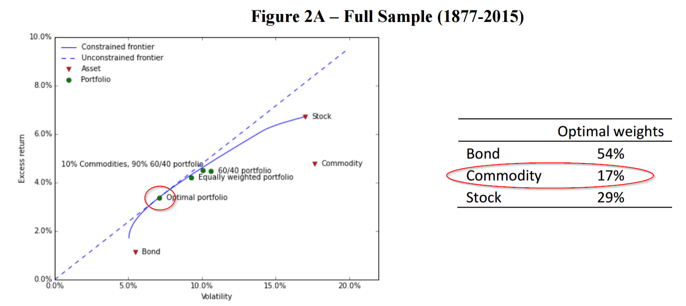
The analysis suggests that even a 10% allocation to commodities adds value over a traditional 60/40 stock/bond allocation. The optimal mean-variance portfolio, which optimizes the Sharpe ratio, suggests the following allocations:

• 17% to commodities, 29% to stocks, and 54% to government bonds.

Over this period, while commodities have offered lower expected returns than stocks, but with similar volatility, their low correlation with stocks and bonds offers potential portfolio diversification benefits.

Summary

Commodity futures are a unique asset class that cannot be replicated via equities, bonds, or equity/bond combos. Commodity futures stand on their own and should at least be considered by investors. The research consensus is that commodity futures’ returns are driven in part by spot price movements and in part by roll yield (or variants such as interest-rate adjusted carry). The disagreement in the research (primarily the quibbles across Erb/Harvey and Gorton/Rouwenhorst) boils down to estimating the expected returns associated with the two components of commodity future returns. The problem is a lack of out-of-sample data.

Thankfully, the AQR team has done the finance research world a service by examining commodity futures returns over a vast time period  (1877-2015) that includes a variety of regimes and non-overlapping time periods. Their findings trump all others and should be considered the “gold standard” until new and better research hits the circuit.

The key takeaways are the following:

• Commodity futures index returns are positive and significant over time.
• Interest rate adjusted carry (convenience yield – storage costs) is responsible for most of the return, arguably earning a “speculator premium.”
• Commodity spot returns drive futures volatility and these returns are positively correlated with macroeconomic states (expansion/recession), suggesting the existence of a risk premium.
• Commodity futures offer an inflation hedge and enhanced returns in “backwardation” markets, highlighting a unique portfolio diversification benefit.

From an investment perspective there are a few things to consider when investing in commodity futures:

• Focus on products that capitalize on net convenience yield.
• Focus on products that equal-weight or volatility-weight allocations versus products weighted based on liquidity or production.

Congratulations on making it this far and let us know if you have any insights or questions. We’ve traded commodity futures for many years and are happy to address any questions you might have.

***Thanks to David Foulke, Gary Antonacci, Andrew Miller, and Mitesh Patel for edits and thoughts.

References[+]

References

↑1	We’ve chosen to deploy these strategies in our own investment strategies. Contact us if you are interested in learning more.
↑2	Many market observers compare the performance of commodity equities to a buy and hold futures strategy that rolls futures. First, blindly buying and holding commodity futures isn’t a viable commodity futures strategy and often ignores roll yield, which often overwhelms the spot return component of a commodity futures contract. Second, any commodity future vs. commodity equity comparisons should be based on collateralized futures, to ensure an apples-to-apples comparison. Finally, there are many reasons why commodity equities may not capture a commodity’s spot return, including idiosyncratic business and production risk, commodity storage costs, and the fact producers often hedge their own production.
↑3	Note the construction of BCOM and GSCI: BCOM: Bloomberg Commodity Index (BCOM) is calculated on an excess return basis and reflects commodity futures price movements. The index rebalances annually weighted 2/3 by trading volume and 1/3 by world production and weight-caps are applied at the commodity, sector, and group level for diversification. The roll period typically occurs from the 6th-10th business day based on the roll schedule. GSCI: The S&P GSCI Total Return Index in USD is widely recognized as the leading measure of general commodity price movements and inflation in the world economy. The index is calculated primarily on a world production weighted basis, composed of the principal physical commodities futures contracts.
↑4	Bhardwaj, Gorton, and Rouwenhorst also point out that the spot returns are not net of storage costs. One can’t simply hold barrels of oil in their backyard. If one were to account for storage costs, the net spot return would more closely mirror the future contract.
↑5	Erb and Harvey (along with Kevin Norrish) would argue that it is unrealistic that lean hog futures receive the same allocation as oil futures.
↑6	“Commodity Investing” by Rouwenhorst and Tang is a good background paper as well
↑7	More complex versions of this formula are available, but we are simply trying to make the point as clear as possible with minimal mathematical notation.
↑8	In the example above we assume that the convenience of owning physical gold was 10%. In reality, we don’t know the convenience yield, we simply know market prices and we can back out the implied convenience yield (similar to backing out implied volatility from option prices). Convenience yield is a benefit to being long commodity futures, whereas interest rates and storage costs are an expected cost of being long commodity futures. Throwing the math aside, this is an intuitive result. If an investor is long a future they are getting an implicit loan and dodging the costs of commodity storage costs — so the future buyer should pay a cost. Of course, a long future investor (who doesn’t own the physical commodity) is also losing out on any convenience yield — so they should get paid a benefit.
↑9	Also note that the situation mentioned does not include the return one might earn on the collateral they maintain to hold the futures contract. In the case of a fully collateralized future (one deposits cash that reflects the notional value of the future), the investor would also earn the risk-free rate (minus a haircut on the rate from the broker). This collateral return could also be included in the return to the future. Hence the reason one will see “excess” future returns and “total” or “collateralized” future return information. Make sure you note which one you are looking at!
↑10	Using the examples from above we came to understand that roll yield is determined by a mix of interest rates (r), storage costs (s), and convenience yields (c). In the AQR paper, Levine et al. leverage more sophisticated mathematics and rearrange the return on commodity futures contracts into two components: erSt,t+1, which is the spot return on the commodity (less the risk-free rate); this is “spot returns in excess of cash.” This is the difference between spot returns and the interest rate. 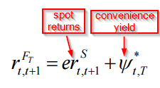ψ*t,T, which is convenience yield less storage costs, or net convenience yield (roll yield plus the short rate), or interest-rate adjusted carry; without this adjustment for interest rates, practitioners refer to this as “carry,” “income,” or “roll yield.” Note the allocation of the “short rate,” which is simply the continuously compounded interest rate. The authors subtract cash rates from the spot returns, and adjust the carry by the short rate. The authors argue this is a more intuitive approach that isolates the effective role of carry in commodity futures returns. A Note on Collateralization The discussion above relates to futures prices. In order to actually implement a futures trading strategy, collateral is required, on both the short as well as the long side. So in a sense, there are two layers of leverage to consider — one layer at the level of embedded interest rates within the futures price themselves, and another layer that is associated with collateralization during trading and implementation. If the investor posts cash to satisfy the collateral requirements, he will earn interest on the collateral (usually a discount to the risk-free rate). By contrast, if he posts, say, equity, to satisfy the collateral requirements, he will borrow against his equity position to create the cash balance required to collateralize his futures position, and he will pay interest on this loan. So depending on the specific situation, collateralization can affect a trading P&L in different ways. The paper under discussion relates to futures prices only and does not consider the effects of collateralization. Other papers, such as Erb and Harvey (2015) and work by Gorton and Rouwenhurst, do consider the effects of collateralization. It’s important to keep these layers of leverage separate for a complete understanding.
↑11	Note that the risk-free rate is being taken out of the spot return in this decomposition. Typically returns are broken into spot and roll yield, where roll yield is convenience yield – storage costs – risk-free rate. The interest rate adjusted carry is deemed to be a more intuitive breakdown of the return to commodity futures.
↑12	Note that, as discussed earlier, this does NOT include the leverage effects of collateralizing a trading position, as explored by Erb and Harvey. By contrast, Levine et al. are focused on the leverage embedded in the futures price itself, and how this should naturally accrue to the carry component, rather than to the spot component. This is a subtle but important distinction that many practitioners fail to grasp, especially when they divide futures returns into spot return and roll yield.