Don’t Make a Bar Bet with Warren Buffett

This past weekend Warren Buffet made some headlines that has the financial world spinning:

• Berkshire Hathaway released its annual report…which is always a great read.
• The (in)famous bet of Buffett’s that the S&P would outperform a basket of hedge funds is almost over (the hedge funds just need to finalize their performance figures for 2016 and the bet will be over).

Mr. Buffett’s bet against hedge funds really intrigued me so I decided to dig a bit further.

Hedge funds, as a whole, have recently received their (more than?) fair share of condemnation from the financial press and analysts as too expensive and too opaque. Pension funds and endowments finally realized they’ve potentially been swindled, and have cut — and even eliminated — their allocation to hedge funds. Clearly, Buffett won the bet.

But Buffet’s victory is easy to see in hindsight. Perhaps the inevitability of the S&P 500 victory over hedge funds wasn’t as clear cut at the time? For example, highly sophisticated investors, such as Cliff Asness, walk through some great portfolio construction points on why hedge funds, as a whole, aren’t as great or as bad as most people make them out to be.

To assess just how smart/lucky Buffett was in making his bet with the hedge funds, in this post, I try and determine what Buffett’s odds really were when he made his famous bet.

Do you really want to bet against Warren Buffett?

Capital Market Expectations and Buffet’s Hedge Fund Bet

In order to judge Buffett’s odds of winning the bet against hedge funds, we first need to develop a set of capital market expectations.  I will develop mine based on history for the S&P 500 and then slightly modify Cliff Asness’s equation for hedge fund returns for my expectation for Hedge Fund returns.

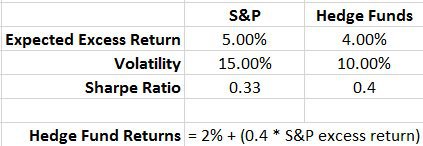
My capital market assumptions are below:

The results are hypothetical results and are NOT an indicator of future results and do NOT represent returns that any investor actually attained. Indexes are unmanaged, do not reflect management or trading fees, and one cannot invest directly in an index.

Historically, the S&P 500 has had a Sharpe ratio of only about 0.33 since 1926 (its actually a little closer to 0.35 but I wanted to make the math easier and end up with round numbers, so I used 0.33).  I assume that the standard deviation for the S&P 500 is 15% per year going forward which makes the excess return (return in excess of cash) 5% per year (Sharpe ratio x volatility = excess return).

Using the equation in Cliff’s article, we assume that Hedge Funds have a beta of 0.4 to the S&P 500 (Cliff shows a beta of 0.37 but I rounded for simplicity and to get whole numbers) and Cliff shows an alpha of 3.65% per year.  I will assume 2% per year as his alpha is backward looking and we need a forward looking expectation.  I assume 2% per year as Hedge Funds are likely to generate some after fee alpha, but not as much as they have historically.  I assume somewhere around half the alpha (1.8% per year) but round up to get to a nice whole number of 2% (did I mention that this is a very scientific and exact analysis?).  This leads to an expectation of a 0.4 Sharpe ratio for Hedge Funds and (I am assuming) a 10% annualized standard deviation.

The end result of these assumptions are that Hedge Funds have a lower expected return than the S&P 500 (4% vs. 5%) even when we assume 2% per year after fee alpha.  In addition, we also assume Hedge Funds are less volatile than stocks (10% vs. 15% standard deviation).  This leads to Hedge Funds having an improved Sharpe ratio versus the S&P 500 (0.4 vs. 0.33).  Hopefully, these set of assumptions can be viewed as moderate and reasonable by both the Hedge Fund supporters and also the passive index fund supporters.

Analysis Method

Now that we have our assumptions, we can analyze the bet by performing a Monte Carlo analysis.  I used Excel to generate a 1,000 random numbers between 0 and 1.  Each number between 0 and 1 was then used as the probability in a normal distribution to create a randomized return (using Excel’s =norminv function) for both the S&P 500 and for Hedge Funds where the mean and standard deviation were equal to the capital market assumptions, above.  Doing the Monte Carlo analysis in this way, it is assumed that that the correlation of the S&P 500 and Hedge Funds are a perfect 1.0 (However, given the very high (~95% correlation) in reality, the assumption of perfect correlation may not be far off).

Analysis Results

What I found is that using the analysis method above, the S&P averaged an excess return of 5.25% over the 1,000 simulations and that Hedge Funds averaged a 4.16% return over the 1,000 simulations.  These results are pretty close to our capital market expectations so randomness inside the 1,000 simulations didn’t move actual results from expected results by much.  What is interesting is that over the 1,000 simulations the S&P beat Hedge Funds in 58.6% of the simulations!  Even though our assumptions regarding Hedge Funds leads us to expect a higher Sharpe ratio (and arguably a better addition to an existing portfolio…see Cliff’s article here for why), the slightly higher expected excess returns from stocks and the lower volatility of Hedge Funds make the S&P 500 a better bet in this type of horse race between investments (perhaps the bet should have been that Hedge Funds would produce a CAPM regression alpha great then 0%!). [bctt tweet=”Don’t bet with Buffett. The S&P 500 beats hedge funds nearly 60% of the time!” username=”alphaarchitect”]

Conclusion

To nobody’s surprise, Warren Buffet had the better end of the deal on this bet (the bet paid even money, while Buffett was arguably expected to win approximately 60% of the time) which is quite the value investment from Mr. Buffett’s perspective.

There are some practical takeaways from this lesson as well:

1. Even though an investment might have a good risk/return trade-off (in this example a Sharpe ratio of 0.40 vs 0.33) and be a great addition to a portfolio (in this example after fee alpha of 2%), it might lose an investment horse race against a passive index more than 50% of the time.  This makes it important to properly select a benchmark for these types of investments to ensure that investors don’t dump them out of frustration when they have poor relative performance.
2. My understanding is that the escrow collateral (a zero-coupon bond) outperformed both the S&P 500 and the Hedge Fund basket selected.  This demonstrates just how important diversification is in portfolios and why a simple 1/N type of allocation might be best. In Buffett’s words, “Beware of geeks bearing formulas.”