In our context, a technical trading indicator can be considered as a combination of a specific technical trading rule with a particular moving average of prices. In two preceding blog posts we showed that there are many technical trading rules, as well as there are many popular types of moving averages. As a result, there exist a vast number of potential combinations of a specific trading rule with a specific moving average of prices. So far, the development in this field has consisted in proposing new ad-hoc trading rules and using more elaborate types of moving averages in the existing rules. Each new proposed rule (or moving average) appears on the surface as something unique. Often this new proposed rule (or moving average) is said to be better than its competitors; such a claim is usually supported by colorful narratives and anecdotal evidence.
The existing situation in the field of market timing with moving averages is as follows. Technical traders are overwhelmed by the variety of choices between different trading indicators. Because traders do not really understand the response characteristics of the trading indicators they use, the selection of a trading indicator is made based mainly on intuition rather than any deeper analysis of commonalities and differences between miscellaneous choices for trading rules and moving averages. It would be no exaggeration to say that the existing situation resembles total chaos and mess from the perspective of a newcomer to this field. Therefore there is an urgent need to bring some order to the chaos in the field of market timing with moving averages.
In this blog post we uncover the anatomy of market timing rules with moving averages of prices. In particular, we are going to show that the computation of a technical trading indicator for every market timing rule can be interpreted as the computation of a weighted moving average of price changes over the averaging window. More formally, we will show that the computation of a technical trading indicator for every market timing rule can be written as

where, recall, ΔPt-i=Pt-i+1-Pt-i denotes the price change and πi is the weight of the price change ΔPt-i in the computation of a weighted moving average of price changes. Therefore, despite a great variety of trading indicators that are computed seemingly differently at the first sight, the only real difference between the diverse trading indicators lies in the weighting function used to compute a moving average of price changes. This result allows us to study the computation of trading indicators in many market timing rules and analyze the commonalities and differences between the rules.
Momentum Rule
The computation of the technical trading indicator for the Momentum rule can be re-written as follows:

Therefore,

where the mathematical symbol “≡” means “equivalence”. To see the equivalence of equations (1) and (2), observe that

(since n-1>0) and vice versa. Consequently, equation (2) allows us to re-interpret the computation of the technical indicator for the Momentum rule as the computation of an equally weighted moving average of price changes (where the weight of each price change equals 1/(n-1)).
Price Minus Moving Average Rule
First of all, recall (from Part 1) the alternative representation of a general moving average:

where wj is the price weighting function and φi is the price-change weighting function of a moving average. Therefore,

Consequently, the computation of the technical indicator for the Price Minus Moving Average rule can equivalently be interpreted as the computation of a weighted moving average of price changes.
In case all weights wj are strictly positive, the sequence of weights φi is decreasing with increasing i

Therefore, in this case, regardless of the shape of the weighting function for prices wj, the weighting function φi always over-weights the most recent price changes.
The closed-form expression for the computation of the technical indicator for the Price Minus Simple Moving Average rule is given by (we skip the details of the derivation)

The resulting formula suggests that we can alternatively interpret the computation of the technical indicator for the Price Minus Simple Moving Average rule as the computation of a Linearly Weighted
Moving Average of price changes.
When the Exponential Moving Average is used in this rule, the closed-form expression for the computation of the technical indicator is given by

In words, the computation of the trading indicator for the Price Minus Exponential Moving Average rule is equivalent to the computation of an Exponential Moving Average of price changes.
For the sake of illustration, the figure below plots the shapes of the price change weighting functions in the Momentum (MOM) rule and three Price Minus Moving Average rules: Price Minus Simple Moving Average (P-SMA) rule, Price Minus Linear Moving Average (P-LMA) rule, and Price Minus Exponential Moving Average (P-EMA) rule. In all rules, the size of the averaging window equals n=30. Observe that in all but the Momentum rule the weighting function overweights the most recent price changes (note that Lag 1 denotes the most recent price change).
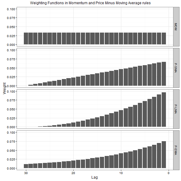
The results are hypothetical results and are NOT an indicator of future results and do NOT represent returns that any investor actually attained. Indexes are unmanaged, do not reflect management or trading fees, and one cannot invest directly in an index. Additional information regarding the construction of these results is available upon request.
The interactive illustration of weighting in the Price Minus Moving Average rule can be found here.
Moving Average Change of Direction Rule
The value of this technical trading indicator is based on the difference between the values of the same weighted moving average computed at times t and t-1 respectively. We assume that in the moving average the size of the averaging window equals n-1. The reason for this assumption is to ensure that the trading indicator is computed over the window of size n. The straightforward computation yields

Consequently, the computation of the technical indicator for the Moving Average Change of Direction rule can be interpreted as the computation of a weighted moving average of price changes. It is worth noting that the weighting function for price changes is virtually identical to the weighting function for computing the moving average of prices.
Three interesting relationships can be derived on the basis of the result above. First, when the Simple Moving Average is used (where wi-1=1 for all i):

where the last equivalence follows from equation (2). Second, when the Linear Moving Average is used (where wi-1=n-i):

where the last equivalence follows from equation (3). Third, when the Exponential Moving Average is used:

where the last equivalence follows from equation (4).
Putting it into words, these relationships mean the following:
- The Simple Moving Average Change of Direction rule is equivalent to the Momentum rule;
- The Linear Moving Average Change of Direction rule is equivalent to the Price Minus Simple Moving Average rule;
- The Exponential Moving Average Change of Direction rule is equivalent to the Price Minus Exponential Moving Average rule.
For the sake of illustration, the figure below plots the shapes of the price change weighting functions in four Moving Average Change of Direction rules: Simple Moving Average (SMA) Change of Direction rule, Linear (LMA) Moving Average Change of Direction rule, Exponential Moving Average (EMA) Change of Direction rule, and Double Exponential Moving Average (EMAEMA) Change of Direction rule. In all rules, the size of the averaging window equals n=30.
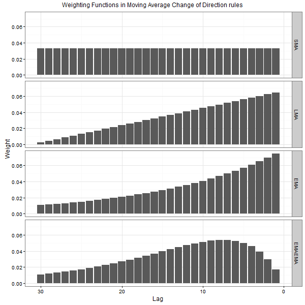
The results are hypothetical results and are NOT an indicator of future results and do NOT represent returns that any investor actually attained. Indexes are unmanaged, do not reflect management or trading fees, and one cannot invest directly in an index. Additional information regarding the construction of these results is available upon request.
The interactive illustration of weighting in the Moving Average Change of Direction rule can be found here.
Moving Average Crossover Rule
Using the alternative representation of a general weighted moving average, the computation of the trading indicator in the Moving Average Crossover rule can be expressed as

where φjl and φjs are the weights of the longer and shorter moving average respectively. Another alternative expression for the computation of the trading indicator in the Moving Average Crossover rule is given by

The computation of the trading indicator in the Moving Average Crossover rule is basically similar to the computation of the trading indicator in the Price Minus Moving Average rule; the only difference is that the shorter moving average is used instead of the last closing price. To understand the effect of using the shorter moving average instead of the last price, we present the computation of the trading indicator in the Price Minus Moving Average rule in the following form (assuming that n=l)

The comparison of equations (5) and (6) reveals that the price change weighting functions for both the rules, MAC(s,l) and P-MA(l), are identical beginning from lag s and beyond. In contrast, as compared to the price change weighting function of P-MA(l) rule, the price change weighting function of MAC(s,l) rule assigns smaller weights to the most recent price changes (from lag 1 to lag s-1). Since most typically the price change weighting function in the P-MA(l) rule overweights the most recent price changes, the reduction of weights of the most recent price changes in the MAC(s,l) rule makes its price change weighting function to underweight both the most recent and the most distant price changes. As a result, in this rule the weighting function for price changes takes a hump-shaped form.
For the sake of illustration, the figure below plots the shapes of the price change weighting functions in four Moving Average Crossover rules: Simple Moving Average (SMA) Crossover rule, Linear (LMA) Moving Average Crossover rule, Exponential Moving Average (EMA) Crossover rule, and Double Exponential Moving Average (EMAEMA) Crossover rule. In all rules, the sizes of the shorter and longer averaging windows equal s=10 and l=30 respectively.
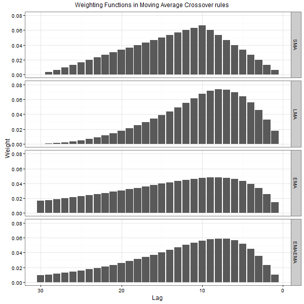
The results are hypothetical results and are NOT an indicator of future results and do NOT represent returns that any investor actually attained. Indexes are unmanaged, do not reflect management or trading fees, and one cannot invest directly in an index. Additional information regarding the construction of these results is available upon request.
The interactive illustration of weighting in the Moving Average Crossover rule can be found here.
Moving Average Convergence/Divergence Rule
The computation of the technical trading indicator of the original MACD rule by Gerald Appel is based on using three Exponential Moving Averages:


For this rule, the computation of the trading indicator, in terms of price changes, is given by (we skip the details of the derivation)
![\text{Indicator}_t^{\text{MACD}(s,l,n)} = \sum_{j=1}^{\infty}\left( \left( \lambda_l^j - \lambda_s^j \right) - (1-\lambda) \left[ \frac{\lambda_l^j-\lambda^j}{1-\frac{\lambda}{\lambda_l}} - \frac{\lambda_s^j-\lambda^j}{1-\frac{\lambda}{\lambda_s}} \right] \right) \Delta P_{t-j},](https://alphaarchitect.com/wp-content/ql-cache/quicklatex.com-6802e58c522f6fbfdc8c6a8183044041_l3.png "Rendered by QuickLaTeX.com")
where

Obviously, the computation of the trading indicator can also be interpreted as calculating a weighted average of price changes. When other types of moving averages is used in this rule, the computation of the trading indicator can again be interpreted as a computation of a moving average of price changes.
The figure below illustrates the shapes of the price change weighting functions in three Moving Average Convergence/Divergence rules where the first, second, and third one are based on SMA, LMA, and EMA respectively. In all rules, the sizes of the averaging windows equal s=12, l=26, and n=9 respectively.
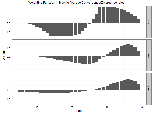
The results are hypothetical results and are NOT an indicator of future results and do NOT represent returns that any investor actually attained. Indexes are unmanaged, do not reflect management or trading fees, and one cannot invest directly in an index. Additional information regarding the construction of these results is available upon request.
Observe that all price-change weighting functions first increase, attain a maximum, then decrease below zero, attain a minimum, and finally increase toward zero. The pattern of the alternation of weights in these functions resembles a damped harmonic oscillator (for example, a sine wave) which suggests that these rules are supposed to react to the changes in the price trend. For example, a strong Buy signal is generated when the prices first trend downward (the price changes are negative), then upward (the price changes are positive). Similarly, a strong Sell signal is generated when the prices first trend upward, then downward. Alternatively, these rules might work well when prices are mean-reverting.
The interactive illustration of weighting in the Moving Average Convergence/Divergence rule can be found here.
Moving Average Envelope
We remind the reader that a moving average envelope consists of two boundaries above and below a moving average MAt(n). The lower (Lt) and upper (Ut) boundaries of the moving average envelope are computed as

where p (usually specified as a percentage) is the distance from the moving average and a boundary of the envelope. The trading signal in the MAE(n,p) rule is generated according to:

It is worth noting that in all previous rules the trading signal is generated on the basis of the value of the trading indicator: positive (negative) value is translated into a Buy (Sell) signal. In contrast, in the MAE rule the trading signal is generated without the computation of the value of the trading indicator. Therefore, for this rule there is no alternative expression for the value of the trading indicator in terms of a weighted average of price changes. However, this fact does not mean that we have absolutely no clue about the shape of the price-change weighting function in the MAE rule. Since the MAE(n,p) rule converges to the P-MA(n) rule when p approaches zero, we have good reason to believe that the shape of the price-change weighting function in the MAE(n,p) rule is close to that in the P-MA(n) rule, at least when p is small.
Summary
Our analysis revealed that all considered technical trading indicators are computed in the same general manner. In particular, any trading indicator is computed as a weighted average of price changes over the averaging window. As a result, each trading rule based on one or multiple moving averages of prices can be uniquely characterized by a single moving average of price changes. Therefore any differences between trading rules can be attributed solely to the differences between their price change weighting functions. As a natural consequence to this result, two seemingly different trading rules can be equivalent when their price change weighting functions are alike.
Our methodology of analyzing the computation of trading indicators for the timing rules based on moving averages offers a broad and clear perspective on the relationship between different rules. Whereas moving averages of prices are indispensable in visualizing how the trading signals are generated, because there is a great variety of trading rules, it is virtually impossible to see the commonalities and differences between various trading rules. In addition, if more than two moving averages are used to generate a trading signal, in this case it is also cumbersome to understand how a trading signal is generated. In contrast, our methodology of presenting the computation of the trading indicator in terms of a single moving average of price changes, rather than one or multiple moving averages of prices, uncovers the anatomy of trading rules and provides very useful insights about popular trend rules. In addition, our analysis offers a new and very insightful re-interpretation of the existing market timing rules.
The list of the useful insights about the popular trend rules, uncovered by our analysis, includes, but is not limited to, the following. First of all, in spite of the fact that there is a great number of potential combinations of a specific trading rule with a specific price weighting function (that is, a moving average of prices), there are only four basic types (or shapes) of price change weighting functions:
- Functions that assign equal weights to all price changes (as in the MOM and ΔSMA rules);
- Functions that overweight the most recent price changes (as in virtually all P-MA rules, ΔMA rules with ordinary moving averages, and the MAE rules);
- Hump-shaped functions that underweight both the most recent and the most distant price changes (as in virtually all MAC rules and ΔMA rules with moving averages of moving averages);
- Functions that have a damped waveform (as in all MACD rules and MAC rules with moving averages with less lag time). Whereas in the previous types of weighting functions all price changes have non-negative weights, in this type the weights of price changes periodically change sign from positive to negative or vice versa.
The other important insights revealed by our analysis:
- The same type of shape of the price change weighting function can be created using several alternative trading rules;
- There are trading rules with exactly the same shape of the price change weighting function; hence these rules are equivalent;
- The trading rules that have either equal, decreasing, or hump-shaped form of the price change weighting function represent the “authentic” trend rules. These rules are designed to generate correct signals when prices trend steadily upward or downward;
- The trading rules that have the damped waveform shape of the price change weighting function are designed to react to the changes in the trend direction. These rules generate correct signals when trend either accelerates or decelerates. Such rules might be profitable when either the price trend often changes its direction or prices are mean-reverting.

About the Author: Valeriy Zakamulin
—
Important Disclosures
For informational and educational purposes only and should not be construed as specific investment, accounting, legal, or tax advice. Certain information is deemed to be reliable, but its accuracy and completeness cannot be guaranteed. Third party information may become outdated or otherwise superseded without notice. Neither the Securities and Exchange Commission (SEC) nor any other federal or state agency has approved, determined the accuracy, or confirmed the adequacy of this article.
The views and opinions expressed herein are those of the author and do not necessarily reflect the views of Alpha Architect, its affiliates or its employees. Our full disclosures are available here. Definitions of common statistics used in our analysis are available here (towards the bottom).
Join thousands of other readers and subscribe to our blog.