Trend-Following: Testing the Profitability of Trading Rules (Part 6)

The difficulty in testing the profitability of trend-following rules stems from the fact that the procedure of testing involves either a single- or multi-variable optimization. Specifically, any trading rule considered in Part 3 has at least one parameter that can take many possible values. For example, in the Moving Average Crossover rule, MAC(s,l), there are two parameters: the size of the shorter averaging window s and the size of the longer averaging window l. As a result, testing this trading rule using relevant historical data consists of evaluating performance of the same rule with many possible combinations of (s,l). When daily data are used, the number of tested combinations can easily exceed 10,000. Besides, there are many types of moving averages (SMA, LMA, EMA, etc.) that can be used in the computation of the average values in the shorter and longer windows. This further increases the number of specific realizations of the same rule that need to be tested. The main problem in this case is not computational resources, but how to correctly perform the statistical test of the outperformance hypothesis.

In the preceding blog post we considered how to test the outperformance hypothesis for a single specific rule. Testing the outperformance hypothesis for a trading rule that involves parameter optimization is much more complicated. In this blog post we review two major types of tests that are used in finance to evaluate the performance of trading rules that require parameter optimization: back-tests (or in-sample tests) and forward tests (or out-of-sample tests). We also describe common pitfalls in testing trading rules.

Back-Testing Trading Rules

In our context, back-testing a trading rule consists in simulating the returns to this trading rule using relevant historical data and checking whether the trading rule outperforms its passive counterpart. However, because each trend-following rule has at least one parameter, in reality, when a back-test is conducted, many specific realizations of the same rule are tested. In the end, the rule with the best-observed performance in a back-test is selected and its outperformance is analyzed. This process of finding the best rule is called “data-mining”.

The problem is that the performance of the best rule, found by using the data-mining technique, systematically overstates the genuine performance of the rule. This systematic error in the performance measurement of the best trading rule in a back test is called the “data-mining bias”. The reason for the data-mining bias lies in the random nature of any statistical estimator. Specifically, recall from the previous blog post that the observed outperformance of a trading rule consists of two components: the true outperformance and the randomness:

The random component of the observed outperformance can manifest as either “good luck” or “bad luck”. Whereas good luck improves the true outperformance of a trading rule, bad luck deteriorates the true outperformance. It turns out that in the process of data-mining the trader tends to find a rule that benefited most from good luck.

Mathematical illustration of the data mining bias is as follows. Suppose that the trader tests many trading strategies. Suppose in addition that the true performance of each trading strategy equals the performance of its passive benchmark. This means that for all trading strategies the true outperformance is zero and, consequently, the observed outperformance is a zero-mean random variable. The trader uses the significance level of p=0.05, that is, 5%. The test of a single strategy is not data mining; when the trader tests a single strategy, the probability of “false discovery” amounts to 5%. In other words, when an active strategy has the same performance as that of its passive benchmark, the probability that the trader finds that the active strategy “beats” its passive benchmark equals 5%.

Now suppose that the trader tests N such strategies. We further suppose that the N observed outperformances are independent random variables. The probability that with multiple testing at least one of these N strategies produces a p-value below the chosen significance level is given by (we skip the details of the derivation)

If in a single test p=5% and N=10, then p_N=40.1%. That is, if the trader tests 10 different strategies, then the probability that the trader finds at least one strategy that “outperforms” the passive benchmark is about 40%. If N=100, then p_N=99.4%. That is, if the number of tested strategies equals 100, then with the probability of almost 100% the trader finds at least one strategy that “outperforms” the passive benchmark. The selected best strategy in a back test is the strategy that benefited most from luck.

To deal with the data-mining bias in multiple back-tests, one has to adjust somehow the p-value of a single test. Researchers have proposed different methods of performing a correct statistical inference in multiple back-tests of trading rules. The majority of these methods are rather sophisticated; practical implementation of these methods requires a deep knowledge of modern statistical techniques.

The main advantage of back-tests is that they utilize the full historical data sample. Since the longer the sample the larger the power of any statistical test, back-tests decrease the chance of missing “true” discoveries, that is, the chance of missing profitable trading strategies. However, because all methods of adjusting p-values in multiple tests try to minimize a Type I error in statistical tests (probability of false discovery), this adjustment also greatly increases the probability of missing true discoveries (Type II error in statistical tests). That is, when a trading strategy with genuine outperformance has a bad luck to be a part of a multiple test where many poor performing strategies are tested, the outperformance of this superior strategy may not be statistically significant.

Forward-Testing Trading Rules

To mitigate the data-mining bias problem in back-testing trading rules, instead of adjusting the p-value of the best rule, an alternative solution is to conduct forward testing. The idea behind a forward test is pretty straightforward: since the performance of the best rule in a back test overstates the genuine performance of the rule, to validate the rule and to provide an unbiased estimate of its performance, the rule must be tested using an additional sample of data (besides the sample used for back-testing the rules). In other words, a forward test augments a back test with an additional validation test. For this purpose, the total sample of historical data is segmented into a “training” set of data and a “validation” set of data. Most often, the training set of data that is used for data-mining is called the “in-sample” segment of data, while the validation set of data is termed the “out-of-sample” segment. In this regard, the back-tests are often called the “in-sample” tests, whereas the forward tests are called the “out-of-sample” tests.

To illustrate the forward testing procedure, suppose that the trader wants to forward test the performance of the Momentum rule MOM(n). The forward testing procedure begins with splitting the full historical data sample [1,T] into the in-sample subset [1,t] and out-of-sample subset [t+1,T], where T is the last observation in the full sample and t denotes the split point. Then, using the training set of data, the trader determines the best window size n* to use in this rule. Formally, the choice of the optimal n* is given by

where M(n) denotes the value of the performance measure (computed over [1,t]) which is a function of the window size. Finally, the best rule discovered in the mined data (in-sample) is evaluated on the out-of-sample data.

In practical implementations of out-of-sample tests, the in-sample segment of data is usually changed during the test procedure. Specifically, after a period of length s≥1, at time t+s, the trader can repeat the best trading rule selection procedure using a longer in-sample period [1,t+s]. Afterwards, the procedure of selecting the best trading rule can be repeated at times t+2s, t+3s, and so on. Notice that, since the in-sample segment of data always starts with observation number 1, the size of the in-sample window increases with each iteration of the selection of best rule procedure. Observe the following sequence of steps in the out-of-sample testing procedure. First, the best parameters are estimated using the in-sample window [1,t] and the returns to the best rule are simulated over the out-of-sample sub-period [t+1,t+s]. Next, the best parameters are re-estimated using the in-sample window [1,t+s] and the returns to the new best rule are simulated over the out-of-sample sub-period [t+s+1,t+2s]. This sequence of steps is repeated until the returns are simulated over the whole out-of-sample period [t+1,T]. In the end, the trader evaluates the performance of the trading strategy over the whole out-of-sample period.

The great advantage of out-of-sample testing methods is that they, at least in theory, should provide an unbiased estimate of the rule’s true outperformance. An additional advantage is that the out-of-sample simulation of returns to a trading strategy, with subsequent measurement of its performance, are relatively easy to do as compared to the implementation of rather sophisticated performance adjustment methods in multiple back-tests.

Pitfalls in Testing Trading Rules

The outperformance generated by a trend following strategy is not stable in time. On the contrary, the outperformance varies greatly over time. The reason for this is twofold. First, a trend following strategy tends to outperform its passive counterpart during bear markets only. Conversely, during bull markets a trend following strategy tends to underperform. Second, the market’s dynamics are changing over time. As a result of these changes, the outperformance of a trend following strategy is also changing. The time-varying nature of outperformance complicates the testing of profitability of trend following rules.

Consider the following example. Statistical theory says that the longer the historical sample, the easier it is to detect profitable trading rules. This property motivates to test the profitability of trend following rules using the longest available sample of data. The monthly data on a broad US stock market index are available beginning from 1800. On the one hand, long history can provide us with rich information about the past performance of trend following rules. On the other hand, if the market dynamics in the distant past are not the same as in the recent past, the performance of trend following rules in the distant past cannot be used as a reliable indicator of their future performance. Our analysis of the dynamics of the growth rate (not adjusted for dividends) of the broad US stock market index over 1857 to 2015 reveals the presence of a major break around 1944. The illustration is provided in the figure below. This figure plots the cumulative return on the index on the log scale. Two straight segments in the figure show the average growth rates of the index before and after the break. After the break, the index has been growing double as fast as before the break.

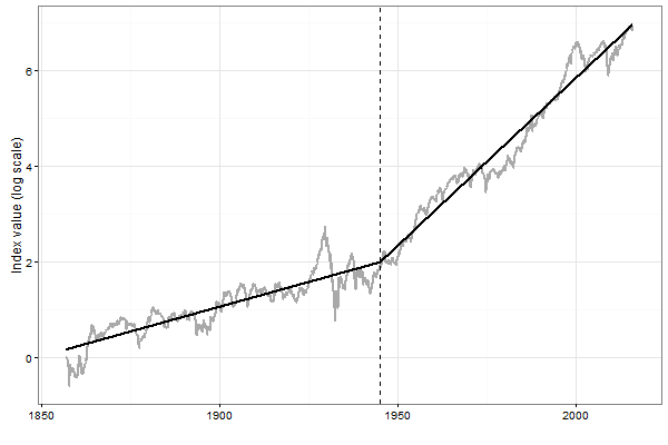
Why is it important to know that in the post World War II era the US stock market index has been growing double as fast as before? The answer is simple: because this structural break in the growth rate of the index affected the dynamics of the bull-bear markets. Specifically, before the break the bull markets were shorter and the bear markets were longer than after the break. As a result, the trend following rules outperformed the passive benchmark to a greater extent before the break than after the break; after the break their outperformance was rather modest. Therefore the historical profitability of trend following rules before the break cannot be used as a reliable indicator of their future profitability; a more reliable indicator of future profitability is their historical profitability in the post World War II period.

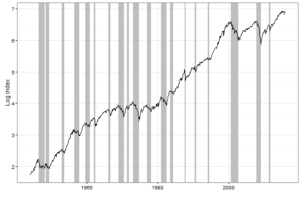
The figure below plots the natural log of the broad US stock market index over the post World War II period. Shaded areas in the figure indicate the bear market phases. It is worth noting that the bull-bear markets are not evenly spaced over time. Therefore in testing the profitability of trend following rules the trader has to ensure that there are enough bull-bear markets in the total sample of data, as well as in both the in-sample and out-of-sample segments of data. A failure of not including both bull and bear periods into the in-sample segment of data results in selecting a trading rule that is not “trained” to detect changes in trends. Similarly, a failure of not including bear periods into the out-of-sample segment of data results in erroneous rejection of “true” discoveries. For example, trend following rules were out of favor before the Dot-Com bubble crash. This is because the long-term pre-crash period, that spans nearly 2 decades, can be regarded as a single long bull market. During that period, in many tests of profitability of trend following rules the out-of-sample segment of data contained the most recent history, the last bull market. As a result, analysts concluded that trend following did not work. They erroneously attributed this finding to “increased stock market efficiency” (recall the Efficient Market Hypothesis which states that technical analysis is useless).

To recap, a trend following strategy tends to outperform its passive counterpart during bear markets only; bear markets are spaced unevenly over time. These two facts complicate the objective testing of profitability of trend following rules and make it possible to manipulate the results of both in-sample and out-of-sample tests. In fact, out-of-sample testing methods have one unresolved deficiency that may seriously corrupt the estimation of the true outperformance of a trend following rule. The primary concern is that no guidance exists on how to choose the split point between the in-sample and out-of-sample subsets. If, for example, the period from 1999 to 2016 (that contains two severe bear markets) is chosen as the out-of-sample segment, then trend following rules appear to be much more profitable than passive investing. In contrast, if one focuses on the most recent history from 2009 to 2016 (where the stock prices have been mainly increasing), then one comes to the opposite conclusion: trend following does not work. Consequently, the choice of the split point can be a decisive factor that determines whether or not a trend following strategy outperforms its passive counterpart.

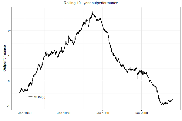
Changing stock market’s dynamics is manifested not only through bull-bear markets. One interesting feature of the stock market dynamics from 1950s to 1990s was the presence of a strong short-term momentum. This short-term momentum was present in all types of stocks; the small cap stocks exhibited the strongest short-term momentum. For the sake of illustration, the figure below plots the rolling 10-year outperformance generated by the MOM(2) rule applied to daily trading a large cap stock index (in the absence of transaction costs). This active strategy is pretty simple: if the index price increases during a day, buy and hold the index. Otherwise, sell the index and place money in cash. Observe that the outperformance of this strategy was increasing until approximately the late 1970s. Then the outperformance of this strategy has been constantly decreasing. Since the early 2000s, the outperformance of this strategy became negative. This fact means that the short-term momentum in stock prices ceased to exist and was replaced by a short-term mean reversion. If, for example, the period from 1960 to date is used as the out-of-sample segment of data, the result of the out-of-sample test leads to the conclusion that the MOM(2) strategy is highly profitable. As a result, one would be tempted to implement this strategy. The consequence of this decision would be a huge loss of money. So the moral of this illustration: do not blindly trust the results of even out-of-sample tests. Because the market’s dynamics are changing, a trend following strategy may lose its profitability. The only possibility to guard yourself against losses is to constantly monitor the recent profitability of a trading rule and see whether this rule performs as it did in the similar situations in the past.

Summary

Each trend following rule has at least one parameter which value is not pre-specified. Many rules have multiple parameters. In practical applications of these rules, the trader has to make a choice of which specific parameters to use. Therefore, traders inevitably tend to search over a large number of parameters in the attempt to optimize a trading strategy performance using relevant historical data. This procedure of selecting the best parameters to use in a trading rule is called back-testing.

However, financial researchers long ago realized that when a large number of technical trading rules are searched, this selection procedure tends to find a rule which performance benefited most from luck. Therefore the observed performance of the best rule in a back-test tends to systematically overestimate the rule’s genuine performance. This systematic error is called the data-mining bias. The methods of correcting the data-mining bias appeared relatively recently. Unfortunately, one can still find recently published papers in scientific journals where researchers employ back-tests and document the observed performance of the best rules without correcting for data-mining bias.

Besides the data-mining correction methods that adjust downward the performance of the best trading rule in a back test, the other straightforward method of the estimation of the true performance of a trading rule is to employ a validation procedure. The method of combination of a back-test with a subsequent validation test is called a forward-test. Another name for this test is an out-of-sample test. As compared to pure back-tests, forward-tests allow a trader to improve significantly the estimation of the true performance of trading rules and these procedures closely resemble actual trader behavior.

However, even though forward-tests are supposed to be purely objective out-of-sample tests with no data-mining bias, in reality there are many pitfalls in conducting the forward tests. These pitfalls may seriously corrupt the validity of results of a forward-test. The two common pitfalls are as follows. First, the market’s dynamics are changing over time. This change in the market’s dynamics influences the profitability of trading rules. To avoid this pitfall requires using the most recent past as the out-of-sample period in a forward test. But here comes the other pitfall: a trend following rule tends to outperform its passive counterpart during bear markets only. The bear markets are spaced very unevenly over time. As a result, the most recent past may contain only a bull market. To avoid this pitfall requires using a sufficiently long out-of-sample period with many bear markets. Quite obviously, it is very difficult for the trader to avoid both pitfalls at the same time!

Past articles in the series are available here.