A few weeks ago, we did a deep dive into the factors versus characteristics debate.
One of the reasons we’ve brought up this debate is due to the fact that “factor” loadings (from regressions) are arguably not as helpful as portfolio characteristics. In other words, knowing a portfolio P/E ratio is more informative for forecasting expected returns than knowing the HML factor loading is .6.
This sentiment is reflected in the paper at hand (“The Cross-Section of Expected Stock Returns” by Jonathon Lewellen. The paper can be found here.):
My paper also relates to Fama and French (1997), Simin (2008), and Levi and Welch (2014), who show that the CAPM and Fama-French (1993) three-factor model do not provide reliable estimates of expected returns. My results suggest that forecasts from characteristic-based regressions have better out-of-sample predictive power than either of the asset-pricing models.
The specific question this paper answer is as follows: Are current firm characteristics predictive of future returns?
Turns out the answer is, “yes.” (at least it was in the past)
This paper uses the Fama-MacBeth (FM) two-stage regression to achieve the average slopes on a variety of commonly-used factor investing strategies. From the average slopes, the paper then goes to examine how well these can be used, with the current characteristics of the firm, to predict future stock returns.
From the abstract, the paper finds that “Empirically, the forecasts vary substantially across stocks and have strong predictive power for actual returns.”
So, given the analysis in the paper, characteristics had predictive power in the past.
Below we dig into the paper.
The Factors, Data, and FM Results
Most are familiar with the numerous factors used by managers/advisors/individuals to sort/screen securities. This paper examines 15 such factors, listed in the paper and described below.
- Size factor = Log market value of equity at the end of the prior month
- Value factor = Log B/M at the end of the prior month
- Momentum factor = Stock return from month -12 to month -2
- Three-year share issuance = Log growth in split-adjusted shares outstanding from month -36 to month -1
- Profitability factor = ROA in the prior fiscal year
- Accrual = Change in non-cash net working capital minus depreciation in the prior fiscal year
- Asset Growth = Log growth in total assets in the prior fiscal year
- Beta = Market beta estimated from weekly returns from month -36 to month -1
- Dividend yield = Dividends per share over the prior 12 months divided by price at the end of the prior month
- One-year share issuance = Log growth in split-adjusted shares outstanding from month -12 to month -1
- Three-year stock return (-36 to -13) = Log stock return from month -36 to month -13
- 12-month volatility = Monthly standard deviation, estimated from daily returns from month -12 to month -1
- 12-month turnover = Average monthly turnover (shares traded/shares outstanding) from month -12 to month -1
- market leverage = Short-term plus long-term debt divided by market value at the end of the prior month
- Sales-to-price ratio = Sales in the prior fiscal year divided by market value at the end of the prior month
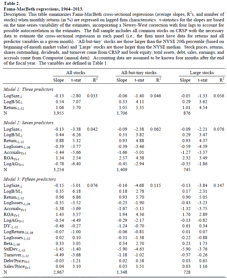
Given the information for all firms, the paper then uses two-stage Fama-MacBeth regression and examines the average slopes (premia). In this paper, the authors test three groups of firms (all stocks, all-but-tiny stocks, and large stocks) from 1964 to 2013 over three models of regressions:
- Model 1– with Three Predictors: size, B/M, and past 12-month stock returns;
- Model 2 — with Seven Predictors: adds three-year share issuance, one-year accruals, profitability, and asset growth;
- Model 3 — with Fifteen Predictors: adds beta, dividend yield, one-year share issuance, three-year stock returns, 12-month volatility, 12-month turnover, market leverage, and the sales-to-price ratio.
Table 2 of the paper shows the results of the FM regressions. Examining both the slopes and the t-stats, we find results that are in line with prior research. Firms with higher B/M ratios, past 12-month returns had higher returns, as evidenced by their statistically significantly positive slopes. Firms issuing more shares, having higher accruals, and more asset growth had lower returns, as evidenced by their statistically significantly negative slopes.
The results are hypothetical results and are NOT an indicator of future results and do NOT represent returns that any investor actually attained. Indexes are unmanaged, do not reflect management or trading fees, and one cannot invest directly in an index. Additional information regarding the construction of these results is available upon request.
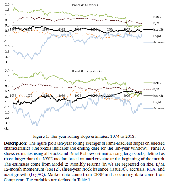
Figure 1 highlights how the slopes from Model 2 change through time (1974 to 2013), using 10-year rolling averages. As we can see, most of the slopes are generally on one side of the y-axis, indicating a positive or negative signal about future returns, such as higher momentum being positive and more accruals being negative. In addition, we see that most of the slopes had relatively steady decline/incline closer to zero, which indicates that past estimates may overstate the cross-sectional dispersion in future returns.
The results are hypothetical results and are NOT an indicator of future results and do NOT represent returns that any investor actually attained. Indexes are unmanaged, do not reflect management or trading fees, and one cannot invest directly in an index. Additional information regarding the construction of these results is available upon request.
Out-of-Sample Predictive Power
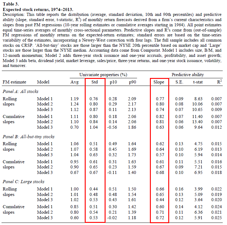
To investigate whether these characteristics persistent predictive power, the paper runs some out of sample tests, first using 10-year rolling average slopes.(1) Table 3 (below) shows the forecasted performance of the three models.
The results are hypothetical results and are NOT an indicator of future results and do NOT represent returns that any investor actually attained. Indexes are unmanaged, do not reflect management or trading fees, and one cannot invest directly in an index. Additional information regarding the construction of these results is available upon request.
What this table is doing is using (1) the past slope estimates and (2) the firm’s current fundamentals, to predict next month’s stock returns. As can be seen in the table below in the univariate properties columns, there is a decent deviation in predicted returns, as evidenced by a monthly standard deviation of ~0.50-0.80%. Examining the 10th percentile, we see that the average predicted monthly return is low (~-0.02-0.40%) for those firms with “bad” characteristics (i.e. low momentum, high accruals, low B/M, etc.) while the 90th percentile has much higher predicted monthly returns (~1.20%-2.00%) for those firms with “good” characteristics (i.e. high momentum, low accruals, high B/M, etc.).
The columns on the right (Predictive ability) come from running FM regressions of monthly realized returns (for all stocks) on expected return estimates (for all stocks), which are again calculated using past slope estimates and current firm’s characteristics. A slope of 1 would indicate that past slopes and current characteristics perfectly describe future returns. As evidenced by the slopes (~0.60-0.80) and t-stats (4+), the returns predicted by current characteristics (and past slopes) do a good job of picking up the variation in future expected returns! Meaning, that firms with good characteristics (in the past), had better returns than firms with bad characteristics. It should be noted that since the slope is not 1, this implies that predicted return estimates should be discounted (by a factor of around 20-40% based on the slopes of 0.80-0.60).
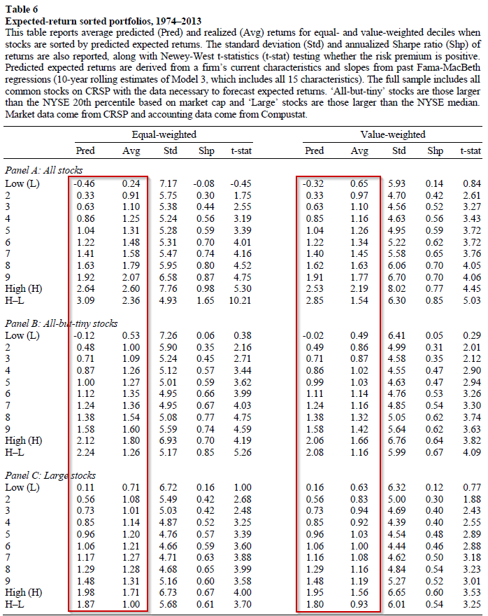
A direct test of how current characteristics could be used to sort stocks is tested in Table 6 of the paper. The paper splits firms into deciles based on their predicted returns (using past slopes and current characteristics).
Results are shown below:
The results are hypothetical results and are NOT an indicator of future results and do NOT represent returns that any investor actually attained. Indexes are unmanaged, do not reflect management or trading fees, and one cannot invest directly in an index. Additional information regarding the construction of these results is available upon request.
The table above shows both the average predicted return and the average realized return to the deciles, using both equal-weighting and value-weighting technique for the deciles. As one can see, there is a monotonic relationship between predicted return deciles and future realized returns (at a monthly level).
Thus, in the past, firms with poor characteristics had poor returns, relative to firms that had good characteristics. The results hold in all samples and using both equal and value-weighting schemes, as evidenced by the t-stats.
Conclusions
This paper asks a simple question–what can current firm characteristics tell us about future predicted stock returns? The answer, using FM regression slopes in the past, is that firms with better characteristics tend to do better in the future. While the expected return estimates using current firm characteristics and past slopes need to be discounted (as they are not perfect), there is a clear relationship (as evidenced in Table 6 of the paper) that firms with better characteristics did better (in the past) than firms with worse characteristics.
However, as with any characteristic-based investing model–it can be simple, but not easy.
The Cross-Section of Expected Stock Returns
- Jonathan Lewellen
- A version of the paper can be found here.
- Want a summary of academic papers with alpha? Check out our Academic Research Recap Category.
Abstract:
This paper studies the cross-sectional properties of return forecasts derived from Fama-MacBeth regressions. These forecasts mimic how an investor could, in real time, combine many firm characteristics to obtain a composite estimate of a stock’s expected return. Empirically, the forecasts vary substantially across stocks and have strong predictive power for actual returns. For example, using ten-year rolling estimates of Fama-MacBeth slopes and a cross-sectional model with 15 firm characteristics (all based on low-frequency data), the expected-return estimates have a cross-sectional standard deviation of 0.87% monthly and a predictive slope for future monthly returns of 0.74, with a standard error of 0.07.

About the Author: Jack Vogel, PhD
—
Important Disclosures
For informational and educational purposes only and should not be construed as specific investment, accounting, legal, or tax advice. Certain information is deemed to be reliable, but its accuracy and completeness cannot be guaranteed. Third party information may become outdated or otherwise superseded without notice. Neither the Securities and Exchange Commission (SEC) nor any other federal or state agency has approved, determined the accuracy, or confirmed the adequacy of this article.
The views and opinions expressed herein are those of the author and do not necessarily reflect the views of Alpha Architect, its affiliates or its employees. Our full disclosures are available here. Definitions of common statistics used in our analysis are available here (towards the bottom).
Join thousands of other readers and subscribe to our blog.