A Q&A Discussion with Vanguard Researchers on the “Fair Value CAPE Ratio”

As everyone who’s been invested for the last ten years knows, post-financial crisis stock returns have been incredible. The chart below highlights the total returns for the S&P 500 Index, the MSCI EAFE Index, the MSCI EEM Index, and the MSCI ACWI Index.

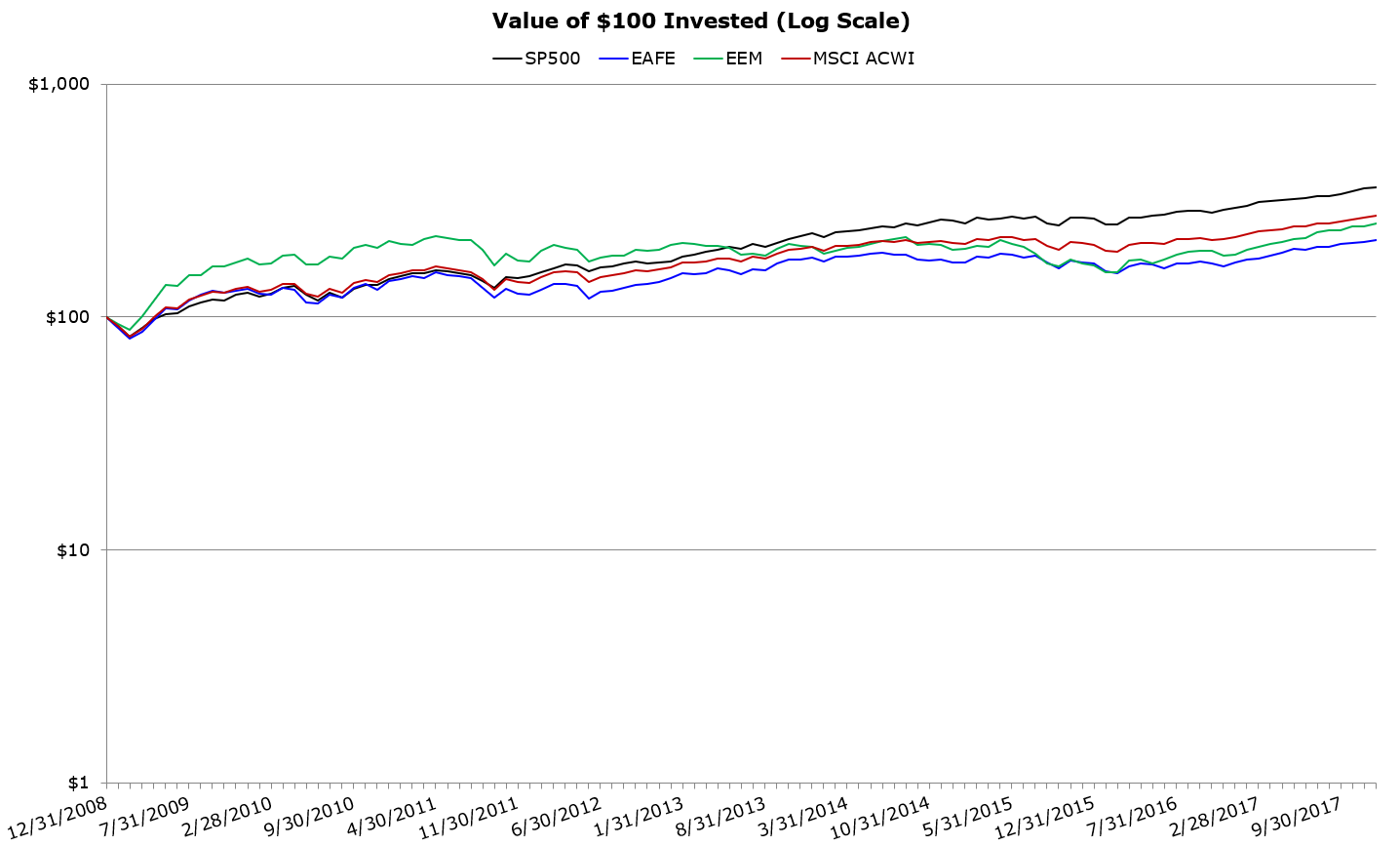
The results are hypothetical results and are NOT an indicator of future results and do NOT represent returns that any investor actually attained. Indexes are unmanaged, do not reflect management or trading fees, and one cannot invest directly in an index.

The market’s gone roughly straight up since 2009. And while some have enjoyed Mr. Market’s sentiment⁽¹⁾, others have consistently vented over seemingly expensive valuations. In many respects, the bull market since 2009 has climbed the proverbial “Wall of Worry.” In other words, at every step up the stock market climb, there have been plenty of reasons for the bull to die along the way.

Source: Ryan Kirlin art studio

Market prognosticators often cite extremely high CAPE ratios (explanation here) as a reason for their angst. This poor sentiment has been vetted via the historical data — high valuations are often associated with low long-term expected returns (see “Jake’s” recent piece).

Here’s a look at the current Shiller-CAPE ratio through the years:

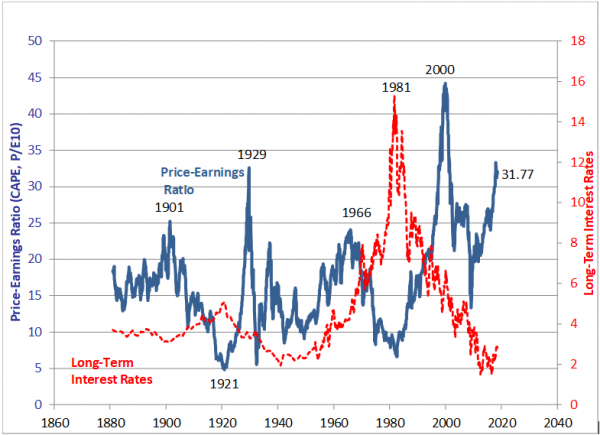
Source: http://www.econ.yale.edu/~shiller/data.htm

There are plenty of reasons why an extreme CAPE ratio may not signal the death of the market, but one can certainly see why investors focused on valuations might be a bit tentative in the current markets — the CAPE ratio is really high relative to historical standards.

But as investors have realized over the past decade, using the CAPE ratio as a tactical allocation tool is difficult at best (see here for a summary and potential solution). Fortunately, there has been a recent research effort at Vanguard to identify better ways to predict futures returns with CAPE ratios (we covered the paper here). Ryan Kirlin and I grabbed one of the authors on the research and sat him down for a discussion on the practical implications of their “fair value CAPE” concept, which seems to be a better predictor of out of sample returns relative to simple CAPE-based solutions.

Can a Vanguard Research Team Improve the Predictive Power of CAPE?

In order to improve upon the CAPE-based forecasting framework, a team from Vanguard’s Investment strategy group began their own research. They published their results in a paper titled,  “Improving U.S. Stock Return Forecasts: A “Fair Value” CAPE Approach.”  We spoke with Roger Aliaga-Diaz, chief economist, North America and principal of the Investment Strategy Group at Vanguard, to learn more about their research and how we can apply it as investors.

Roger Aliaga-Diaz, Senior Economist, Vanguard Group

Wes/Ryan:  First, let’s start out with an easy question: What does CAPE stand for and how is the CAPE ratio used?

Roger: The cyclically adjusted price/earnings (P/E) ratio, proposed by professors John Campbell and Robert Shiller, is a popular equity market valuation metric.  Historically, a high CAPE ratio on average has been associated with low equity returns over the following decade and vice-versa. Thus the CAPE ratio is typically used by practitioners to forecast long-term equity returns.  More specifically, the 10-year ahead returns are regressed against the CAPE at the beginning of the 10 year period and is commonly used to forecast returns for the next decade.

Wes/Ryan:  What drove you and your colleagues to begin researching ways to improve the CAPE ratio?

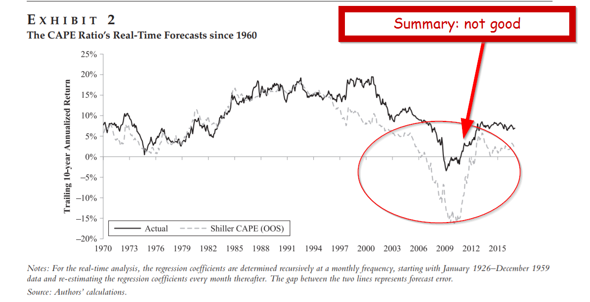
Roger: CAPE and other similar equity valuations metrics have been widely used by practitioners and investment professionals in the asset management industry for at least 10 years or more. Academics have also studied extensively the predictability of CAPE and other metrics. We have been following both streams of work, and we concluded that academics’ predictability tests were more realistic than the practitioners’. Practitioners’ back testing often suffers from a “look-ahead” bias. Academic studies are designed to replicate real time equity forecasts, that is, they simulate an investment professional forecasting equity return in real time, with the data and models available until each point in time. We followed their approach.

In doing so we noticed that the original forecast accuracy of the original CAPE regression was very poor when used in real-time forecasts. In general, the lower the average forecast error, the more accurate a model is.  We estimated the average forecast error (more specifically, the root mean squared error or RMSE) of 10-year annualized return using the CAPE regression in real time, since 1985, to be 7.8%, which is extremely high – in other words, a sign of a poor model performance.

The results are hypothetical results and are NOT an indicator of future results and do NOT represent returns that any investor actually attained. Indexes are unmanaged, do not reflect management or trading fees, and one cannot invest directly in an index.

Moreover, if one were to use a poor forecasting model like a naïve long-term historical average return, the average error was found to be 6.2% which is much lower than the CAPE regression. In order to improve the predictability of returns, we decided to explore models which would reduce the problems associated with the CAPE regression.

Wes/Ryan:  You call your modified CAPE ratio a “Fair-Value Cape Ratio.” Can you contrast that with the other more popular measures of the CAPE ratio (such as the Shiller CAPE)?

Roger: The traditional CAPE regression essentially determines the valuation of the equity market (over or under valued) relative to the historical average level of the CAPE. If CAPE ratio is higher than its historical average, the market is said to be over-valued and vice versa. The first problem with identified with that approach is that a “normal” equity market valuation depends very much on the broader market and economic environment.  For instance, it’s well known among practitioners that low earnings or dividend yields are to be expected during periods of low interest rates. Low earnings yields means high price-earning ratios, but that doesn’t mean the market is over-valued. So, in the fair value CAPE model, we statistically adjust the historical relationship of the CAPE ratio to various economic fundamental variables such as real interest rates, inflation, equity volatility, bond volatility and then forecast these variables 10 years out.

There are additional econometric problems with the traditional CAPE regression: practitioners typically derive a statistical relationship between the 10-year annualized equity returns and initial P/E (i.e. fit a regression line) using quarterly or monthly data. The use of overlapping data (i.e. 10-year returns sampled at monthly frequency) biases dramatically the accuracy of the back tested estimates, giving a false sense of forecast accuracy to the analyst. (editor note: see AQR paper here for a discussion on this point). Applying that biased model to our real-time equity return analysis one can see the dramatic underperformance of those forecasts. Our “fair-value CAPE” is designed to avoid using overlapping data and thus it is unbiased.

Specifically, we forecast 10-years out the “fair-value” CAPE ratio (along with real interest rates, inflation, etc), as opposed to forecasting directly the 10-year annualized equity returns using monthly data like in the traditional Shiller CAPE approach. We then impute equity returns out of our CAPE ratio forecasts using a well-known identity between earnings yields and equity returns:

equity returns = dividend yield (or CAPE times payout ratio) + CAPE expansion (% change in CAPE) + a long-term average earnings growth.

Wes/Ryan:  You say in your paper that “real-time investors would have been better served by using the historical average return as the baseline forecast of future stock returns over the past decade.” So the simplest method was the best???

Roger: Yes; since the average forecast error of a naïve long term historical average return model was lower than that of the traditional CAPE regression, investors may have been better served by using the naïve long term historical average return as a forecast on a relative basis. We estimated the average forecast error of 10-year annualized return using the CAPE regression in real time, since 1985, to be 7.8%, which is extremely high – in other words, a sign of a poor model performance. In contrast, simply assuming the long term historical average return for the next 10 years would have produced a lower average error of 6.2%. Our fair value CAPE model has an average forecast error of  4.1%, which was statistically lower than the naïve long term historical average return model. Thus the fair value CAPE model could be effectively used in forecasting long  term returns and subsequently in asset allocation, which requires forecasted returns as an input.

Wes/Ryan:  Another quote from the paper is, “Siegel [2016] argued the rise in the CAPE’s trend is primarily due to changes in accounting standards over time and the NIPA earnings should be substituted for generally accepted accounting principles earnings when applying the CAPE ratio.”   What do you believe will enable your, “Fair Value Cape Ratio,” to persist in the future where others have recently performed more poorly?

Roger: For the S&P 500 index, the Shiller CAPE divides the current price with trailing 10-year inflation adjusted, reported earnings (GAAP adjusted). Professor Jeremy Siegel, argues that the secular rise in the CAPE ratio is due to changes in accounting standards and replaced GAAP adjusted earnings with NIPA earnings instead. Our research indicated that the average forecast error using Siegel CAPE was not statistically any better than the naïve long term historical average return model for the same period mentioned above. Rather than changing the definition of earnings in the CAPE ratio (as is very common in the literature) we identified weaknesses and biases stemming from a too simplistic CAPE formulation (both Shiller’s and Siegel’s) and develop a more robust statistical framework that doesn’t rely that can better withstand the test of changes in the economic environment over time.

In our view, the weak predictability of the CAPE regression (using CAPE ratio) may be less about the earnings used in the calculation of the ratio (as proposed by Siegel) and more a reflection of model bias and inherent instability. The CAPE regression instability originates from at least two sources. The first is the estimation bias that arises when persistent (or slow moving) variables such as CAPE ratio are used to forecast long run returns. The second relates to the standard CAPE regression omitting the relationship between the earnings yield (or 1/CAPE) and other economic factors like real interest rate as well as inflation and equity and bond volatility. The benefit of our approach is that the value to which the CAPE ratio reverts to (fair value CAPE ratio), is permitted to vary over time, conditional on the other fundamental variables. It is this fair value CAPE that should be the relevant benchmark for forecasting equity returns, not the long run average CAPE which is implicit in the CAPE regression.

Wes/Ryan:  You hypothesize the following: “Lower real bond yields should imply lower earnings yields and thus higher equilibrium or fair value CAPE Ratios, all else equal.” And you also mention your fair-value CAPE ratio varies over time based on three main things: 1.) The state of the economy (as measured by real interest rates), 2.) expected inflation and 3.) measures of financial volatility. Assuming we’re in a rising interest rate environment, what does your model predict for the future?

Roger: A real (not nominal) rise in interest rates, all else equal, would result in lower future CAPE levels and lower equity returns as the CAPE ratio falls. One could also expect some offset by higher earnings growth, which should accompany higher real rates. In other words a small rise in real rates could have a minor impact of lower long run returns, while the impact of a large real rate rise could be more drastic. We do expect the rise in real rate to be small, given the drag of demographics, technology and globalization on global growth as described in the Vanguard Economic and Market Outlook.

Wes/Ryan:  The potential benefit of your approach is that the fair-value CAPE ratio is permitted to vary over time. What type of market could shock your model and cause it to break (at least temporarily)?

Roger: Several shocks could cause a model to break. As an example, extreme shocks in asset prices occurring during the end of 10-year forecast horizon (thereby not allowing the equity market to recover) could cause large forecast errors temporarily. Additionally, temporary disconnect in asset prices (periods of extreme over or under-valuation) could cause the forecasts to have large errors, but we would expect the asset price disconnect to restore to normalcy over the long-term.

Wes/Ryan: Thanks Roger, for your insight and the practical implications of your research. We look forward to more work from Vanguard!