Consider a market-timing strategy which supposedly predicts the direction of the stock market trend. Such a strategy generates Buy and Sell signals. A Buy signal is the signal to buy stocks, whereas a Sell signal is the signal to sell.
Simple enough, but how does one evaluate the forecast accuracy of the market timing strategy?
Quant traders often evaluate the forecast accuracy of a market-timing strategy using a procedure that shows that the strategy accuracy is better than a random guess. Specifically, quant traders often assume that if the accuracy of a market-timing strategy is better than the accuracy of a fair coin, then the strategy has genuine predictive ability.
The typical procedure is implemented as follows:
- Using selected historical data, simulate the market timing strategy and estimate its accuracy.
- Then use the same data to evaluate the accuracy of the strategy based on flips of a fair coin. In particular, for every next period the random strategy generates Buy and Sell signals with equal probability of 50%.
- The statistical inference is conducted by simulating the random strategy, say, 1,000 times. In the end of this procedure, the p-value of the null hypothesis about the equal predictive abilities (of the market timing and the random strategies) is computed by counting the percentage of times the accuracy of the random strategy happens to be better than the accuracy of the market-timing strategy.
There is a potential problem with the framework mentioned above — the results may be erroneous!
Assessing Market-Timing Strategies
The goal of this blog post is to demonstrate that in the presence of a positive long-term market trend, every trading strategy with a long position bias outperforms the 50/50 random strategy. Even if the market-timing approach has zero predictive ability.
First, consider a simple theoretical illustration:
- Let p denote the probability that the one-period market return is positive.
- The probability of a negative market return is, hence, 1-p.
Let us compute the accuracy of the 50/50 random strategy. When this strategy generates a Buy signal, the probability of the correct forecast is 0.5*p. When this strategy generates a Sell signal, the probability of the correct forecast is 0.5*(1-p). The total forecast accuracy is the sum of these two probabilities which is 0.5*p+0.5*(1-p)=0.5. Note, that regardless of the probability of the positive market return, the expected forecast accuracy of the 50/50 random strategy is 50%.
Now suppose that we flip a coin, which is not fair.
In particular, this coin generates Buy and Sell signals with probabilities of q and (1-q) respectively. It is worth emphasizing that our coin has no forecasting abilities at all. Using the same approach to evaluate the forecast accuracy of a non-fair coin, we arrive to the accuracy of q*p+(1-q)*(1-p)=1-p+q(2p-1). Now the forecast accuracy of the random strategy depends on the values of q and p. Only when p=50% is the choice of q irrelevant. It is also relatively easy to see that the forecast accuracy of the random strategy is increasing with respect to q, if p>50%. In particular, if p>50% and q>50%, then the forecast accuracy of the random strategy is greater than 50%. It is important to note that in this case (when p>50%) the maximum forecast accuracy of the random strategy is achieved when q=100%. That is, the buy-and-hold strategy, which can be considered as the random strategy that generates a Buy signal with probability of 100%, has the maximum forecast accuracy among all random strategies with no predictive abilities.
To make this more concrete, consider the long-term data on the S&P 500 index. We know that over the long run that US stocks have gone up. Over a month, the probability that the return on the S&P 500 index is positive is around 60%. Hence, the probability of negative return is 40%. The accuracy of the 50/50 random strategy is always 50%. Suppose now that a market timing strategy has no predictive ability but has a long position bias. That is, it generates a random Buy signal more often than a random Sell signal. If it generates a Buy signal with probability of 70%, then the accuracy of this strategy (with no predictive ability) is 54%, which is better than the accuracy of the random strategy based on a coin flip. If a market timing strategy generates a random Buy signal with probability of 90%, then the accuracy of this strategy will be 58%. Finally, in this case the buy-and-hold strategy with no predictive ability has accuracy of 60%.
A Concrete Example
Let us now consider a specific example. Suppose we hypothesize that the monthly change in the Consumer Price Index (CPI) is able to forecast stock market trends. We decide to run a back-test of this strategy. We find the monthly data on the CPI in the Fred database and the monthly return data on the US stock market in the Ken French data library. Our historical period is from January 1960 to December 2018.
Formally, our strategy is as follows:
- If the monthly change in the CPI is positive, the signal is Buy, otherwise the signal is Sell.
- The computed accuracy of this strategy is 57%, which is higher than the 50% accuracy of a fair coin.
“To be on the safe side” we simulate the 50/50 random strategy 1,000 times and evaluate its accuracy. The result is as follows: In 1,000 simulations the maximum accuracy of the random strategy is 56% and the minimum accuracy is 44%. Based on the simulations, it looks like we are ~100% sure that the CPI has a genuine forecast accuracy relative to a fair coin (57% vs. the best effort of 56% from the simulations).
Unfortunately, the conclusion from the back-test is false. Over the period from January 1960 to December 2018, the monthly market return was positive 62% of times. Thus, any random strategy which generates a Buy signal with a probability greater than 50% will “outperform” a fair coin. Specifically, over the sample period the monthly change in the CPI was positive 88% of times. Clearly, a market timing strategy based on CPI changes has a long bias. Thus, it is not correct to compare the accuracy of the CPI-based market timing strategy with the accuracy of a fair coin.
Let us now compare the accuracy of the market timing strategy with the accuracy of the buy-and-hold strategy. The buy-and-hold strategy always generates a Buy signal and its accuracy amounts to 62%. Even though its accuracy is only marginally higher than the accuracy of the market timing strategy based on the CPI change, the annualized Sharpe ratio of the buy-and-hold strategy is 0.42, whereas the Sharpe ratio of the market timing strategy is 0.31, which is notable lower.
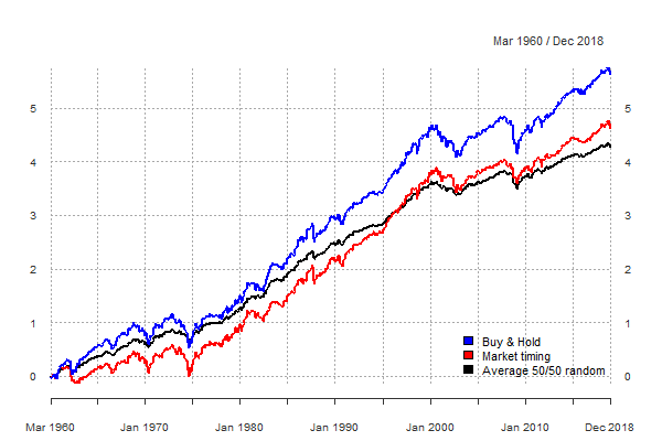
The figure below plots the cumulative returns to the buy-and-hold strategy, the CPI-based market timing strategy, and the average cumulative return to the 50/50 random strategy. The buy-and-hold strategy not only has a higher Sharpe ratio than the market timing strategy, but also higher long-term growth rates. Thus, the buy-and-hold strategy outperforms our market timing strategy. The strong performance of the buy-and-hold strategy comes from the fact that it correctly predicts all positive return observations by construction (and incorrectly all negative returns!). In contrast, our market timing strategy predicts with a limited accuracy both the positive and negative returns.
The results are hypothetical results and are NOT an indicator of future results and do NOT represent returns that any investor actually attained. Indexes are unmanaged and do not reflect management or trading fees, and one cannot invest directly in an index.
Some quant traders do sometimes discover that a market timing strategy, which is better than the 50/50 random strategy, underperforms the buy-and-hold strategy. They believe that this result is counter-intuitive and try to find a feasible explanation for this effect. But the only correct explanation for this effect is that the stock market had a positive trend over the sample period.
Conclusion
The conclusion that can be drawn from the examples in this blog post is pretty obvious. In the majority of financial markets the prices go upward over the long run. Therefore, quant traders must be aware of the fact that every trading strategy with no predictive ability, but a long position bias, tends to outperform the 50/50 random strategies, which are often used as a benchmark for comparison.
An alternative explanation of the effects of the market trend and the position bias on the performance of a market-timing strategy is presented in Aronson (2006), Chapter 1.(1) Aronson suggests that researchers detrend the return data in order to remove the position bias. However, there is no guarantee that after detrending the data the trading signals will be the same as prior to detrending.
Another potential solution is to use the buy-and-hold strategy as the benchmark for comparison. That is, instead of comparing the accuracy of the market timing strategy with the accuracy of the 50/50 random strategy, researchers should compare the accuracy of their market timing strategies with the accuracy of the buy-and-hold strategy.(2)
Thoughts? Ideas? Let us know.

References[+]
| ↑1 | Aronson (2006) “Evidence-Based Technical Analysis: Applying the Scientific Method and Statistical Inference to Trading Signals”, Wiley, can be found here. |
|---|---|
| ↑2 | Techniques for conducting statistical inference are described in Zakamulin (2017), Chapters 7 and 8. Zakamulin (2017) “Market Timing with Moving Averages: The Anatomy and Performance of Trading Rules”, Palgrave, can be found here. |
About the Author: Valeriy Zakamulin
—
Important Disclosures
For informational and educational purposes only and should not be construed as specific investment, accounting, legal, or tax advice. Certain information is deemed to be reliable, but its accuracy and completeness cannot be guaranteed. Third party information may become outdated or otherwise superseded without notice. Neither the Securities and Exchange Commission (SEC) nor any other federal or state agency has approved, determined the accuracy, or confirmed the adequacy of this article.
The views and opinions expressed herein are those of the author and do not necessarily reflect the views of Alpha Architect, its affiliates or its employees. Our full disclosures are available here. Definitions of common statistics used in our analysis are available here (towards the bottom).
Join thousands of other readers and subscribe to our blog.