Early in the summer, I was on a podcast with Corey Hoffstein discussing momentum investing. During the discussion, Corey asked me a question regarding risk versus mispricing, specific to the momentum anomaly. We frequently cite the behavioral explanation for momentum–investors tend to underreact to new information–whereby winning stocks do not go up by as much as they should, given the new “good” information, and losing stocks do not go down by as much as they should, given the new “bad” information. However, a standard debate in empirical asset pricing (academic finance) generally revolves around explaining anomalies through the risk versus mispricing lens.
Thus, what is the risk-based explanation for momentum?
It was a good question Corey asked. My response, around the 12:45 mark in the podcast, was rather short and probably needs more explanation. I walked through the logistics of running a pure long/short momentum portfolio and described some of the risks of running a short portfolio. My logic (in my head) was to tie this to a crash risk component (such as here); however, that was not done too well on the podcast.
So I wanted to dig deeper into the “risk” explanation for the momentum premium. Initially, and not surprising, I found an AQR article “Explanations for the Momentum Premium.” While there is no definitive answer to the risk versus mispricing argument (hence the ongoing research on the topic), the paper does give a good background on some of the risk-based explanations for momentum. From the article:
There is strong correlation structure among momentum stocks. High momentum stocks covary strongly among each other and low momentum stocks covary among themselves, too. This “factor structure” for momentum is at least as strong as that of value or size, which many advocates for value and size (e.g., Fama and French) claim is evidence of a risk-based story. The strong correlation structure for momentum extends across international markets and even across asset classes. A momentum strategy in equities is not only strongly correlated across international markets, but also strongly correlated with one in government bonds, commodities, and currencies. This provides more evidence of the strong covariation or factor structure among assets experiencing momentum which is consistent with a risk-based explanation (Asness, Moskowitz, and Pedersen (2010)).
Why does the covariance structure matter? The genesis of this risk-based explanation is Fama and French (1993).(1) They write:
If assets are priced rationally, variables that are related to average returns, such as size and book-to-market equity, must proxy for sesitivity to common (shared and undiversifiable) risk factors in returns. The time-series regressions give direct evidence on this issue. In particular, the slopes and R^2 values show whether mimicking portoflios for risk factors related to size and [book-to-market] capture shared variation in stock and bond returns not captured by other factors.
Thus, a high covariance (and thus Betas) according to Fama and French (and academics thereafter) implies that there is an undiversifiable common risk amongst the stocks (or bonds). In general, the standard argument of risk versus mispricing centers itself on covariances (risk) versus characteristics (behavior), see here.
Building upon the known strong correlation structure amongst high and low momentum stocks, the 2013 Journal of Finance paper, “Value and Momentum Everywhere” by Asness, Moskowitz, and Pederson (Hereafter AMP) finds the following:
Most strikingly, we discover significant comovement in value and momentum strategies across diverse asset classes. Value strategies are positively correlated with other value strategies across otherwise unrelated markets, and momentum strategies are positively correlated with other momentum strategies globally. However, value and momentum are negatively correlated with each other within and across asset classes.
So not only are momentum stocks highly correlated, but the momentum strategies (long high momentum, short low momentum) are also correlated across other asset classes! Thus, there is something unique about the momentum risk, as there are high correlations both in and across asset classes.
Thus, based on the correlations amongst the Momentum portfolios (for stocks, as well as bonds, commodities, and country indices), the momentum portfolios appear to have a common unknown risk factor (and the same applies to Value). This is a better answer to the question Corey originally asked.
However, what is this “risk”?
For many, including myself, this is always an interesting question. What is/are the risk(s) that are common to Value and Momentum stocks?
A neat paper, which I would like to highlight below, attempts to answer this question for both Value and Momentum. The paper is written by Cooper, Mitrache, and Priestley, and is titled “A Global Macroeconomic Risk Model for Value, Momentum, and Other Asset Classes.” A link to the paper can be found here.
At the outset of the paper, they highlight the results from the “Value and Momentum Everywhere” paper and state the goal of their paper (tying the Value and Momentum premia to macroeconomic variables):
Asness, Moskowitz, and Pedersen (2013) find consistent return premia on value and momentum strategies across both asset classes and countries. They uncover three puzzling findings. First, these return premia are negatively correlated. Second, in spite of this negative correlation, a simple equal-weighted combination of value and momentum produces a positive return premium. Third, various risk factors such as the market portfolio excess returns and liquidity cannot explain these return premia. Instead they rely on global value and momentum factors to describe value and momentum characteristic sorted portfolios. It is not clear though how these factors relate to macroeconomic state variables.
In addition to attempting to tie the “risks” to macroeconomic variables, they highlight a dilemma–(1) Value and Momentum both have positive premia and (2) are negatively correlated, yet (3) the combination produces a positive premium!
Why is this a dilemma? Well, on a standalone basis, Value and Momentum each have positive premia, which means that each has a loading on some unknown macroeconomic risk factor(s) (given the correlation structure). However, since they are negatively correlated, this should mean that Value loads positively on one macroeconomic factor while Momentum loads negatively (or vice versa). However, when combined, the Value and Momentum combination has a positive premium while loading on risks in opposite directions? So how is this possible?
Below we dig into the paper to see how the authors:
- Tie the Value and Momentum risks to macroeconomic variables.
- Explain how Value and Momentum (while negatively correlated) can have a combined positive premium.
Let’s dig in.
The paper set-up
The paper begins by giving a background on the evidence for factors within different asset classes (stocks/ bonds/commodities) and different locations (i.e. the U.S. or International). Some examples are the beta factor, the carry factor, and the size factor. In addition, as evidenced in the “Value and Momentum Everywhere” paper, there are the Value and Momentum factors.
The paper uses the “Value and Momentum Everywhere” datasets, which can be found here. The data is constructed by examining 8 asset classes:
- U.S. Stocks
- U.K. Stocks
- Continental Europe Stocks
- Japanese Stocks
- Country Equity Index Futures
- Currencies
- Government Bonds
- Commodity Futures
From the Value and Momentum Everywhere paper, the equity portfolios are built by only examining the largest firms, as all those that cumulatively account for 90% of the market capitalization (in each respective market). Here are some of the summary statistics:
The U.S. and U.K. stock samples begin in January 1972. The Europe and Japan stock samples begin in January 1974. The average (minimum) number of stocks in each market over their respective sample periods is 724 (354) in the United States, 147 (76) in the United Kingdom, 290 (96) in Europe, and 471 (148) in Japan.
I give this information to highlight the fact that the portfolios all contain very large (and liquid) stocks.
Within each of the 8 asset classes, the authors split the universe into 3 portfolios on either (1) Value and (2) Momentum.(2) The data runs from January 1982 through June 2010.
Now that we have the background on the data, let’s get back to the original question of the paper–Can we tie the Value and Momentum premia to macroeconomic factors?
Well first off, we need to come up with a set of macroeconomic risks (variables) that may influence returns in our asset classes. The authors go back to those outlined in Chen, Roll, and Ross’ 1986 paper, “Economic Forces and the Stock Market” in The Journal of Business (hereafter this paper and the factors will be referred to as CRR). A link to the paper can be found here. The authors find (in their tests) that the macroeconomic risks (described below) are priced in the stock market. So what are the macroeconomic risks that they find are priced in there paper? There are five variables which are listed below (variable abbreviation in parentheses):
- Industrial Production Growth (MP)
- Unexpected Inflation (UI)
- Change in Expected Inflation (DEI)
- Term Spread (UTS)
- Default Spread (UPR)
So how can we test how (and if) the Value and Momentum factors load on these macroeconomic risk factors?
Simply running a regression of the time-series of portfolio returns against the macroeconomic factors creates issues, as some of the factors are noisy with some information not relevant for prices of certain assets (as well as three of the factors being non-tradable!). So to alleviate this concern, the authors use a standard methodology to create a “mimicking” portfolio. High-level, the authors use the six-factor portfolios from the AMP paper.(3) From there, they regress the six-factor portfolios (low, middle and high Value as well as low, middle and high Momentum) on the five CRR macroeconomic factors. The Lehmann and Modest (1988) method does the following:
This methodology produces unit-beta mimicking portfolios, that is, the mimicking portfolio for a specific factor has a beta of unity with respect to that factor and a beta of zero with respect to all other factors.
Again for those interested in the details, please see the paper on pages 10-12.
So high-level, what does this “mimicking” portfolio do?
It generates”weights” (i.e. betas) for the macroeconomic variables once regressed upon the six AMP factor portfolios. Thus, we have taken the six AMP factor portfolios (six Value and Momentum return series on numerous asset classes), regressed these on the macroeconomic factors to get beta loadings, and then used the beta loadings alongside the six AMP portfolios to generate a new return time series for each of the five macroeconomic factors (derived from the six AMP return series) … pretty simple, right!?
So long-story-short, we have now created five new time-series returns for each of the macroeconomic factors.(4)(5)
It is important to understand that for the majority of the paper, we generally will examine the Value and Momentum loadings on the macroeconomic “mimicking” portfolios.
So after the sidetrack into “mimicking” portfolios, we can finally address the initial question–Can we test how (and if) the Value and Momentum factors load on these macroeconomic risk factors?
Yes!
We can examine how the Value and Momentum portfolios load on each macroeconomic factor, within each asset class. This is done by regressing the value and momentum long/short premia (within each test universe) on the mimicking portfolios for each of the macroeconomic factors (the five CRR factors).
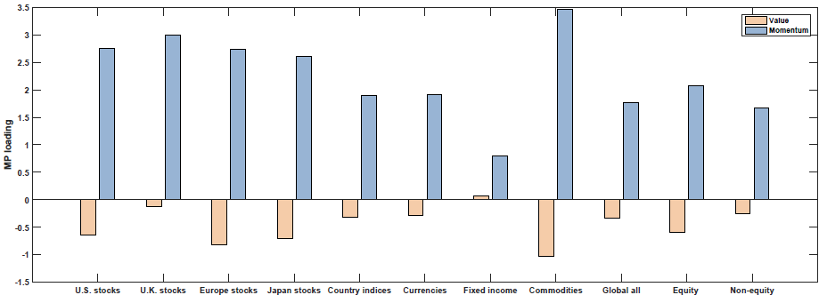
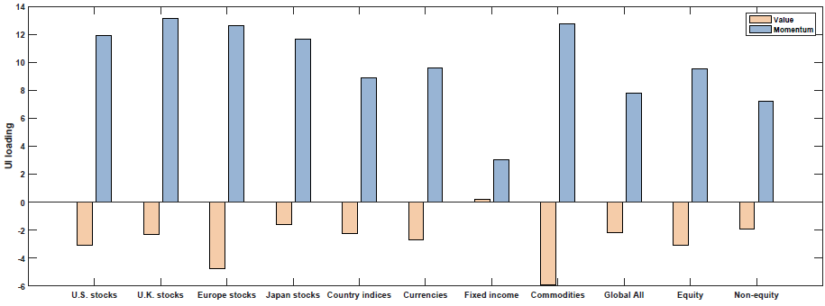
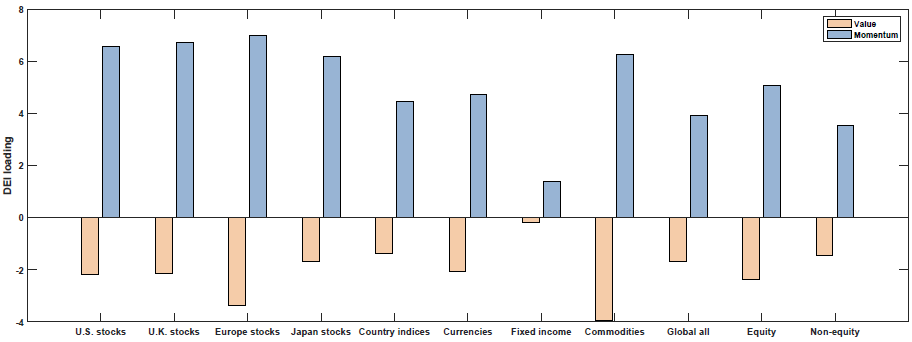
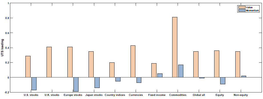
The results are shown in Figure 3 of the paper (as well as Table 5). Below are the results with the blue (yellow) bar representing the loading on each macroeconomic factor for the Momentum (Value) portfolios:
Growth Rate of Industrial Production (MP)
Unexpected Inflation (UI)
Change in Expected Inflation (DEI)
Term Spread (UTS)
Default Spread (UPR)
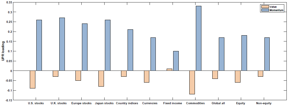
So what we see above is that Value and Momentum load oppositely (in general) on each macroeconomic risk factor! Above we see that Value (Momentum) appears to load positively (negatively) on the Term Spread factor (UTS), while Value (Momentum) loads negatively (positively) on the other 4 macroeconomic risk factors.
Remember at the outset, the paper attempted to answer two questions–(1) tie the Value and Momentum risks to macroeconomic factors/risks, and (2) Explain how Value and Momentum (while negatively correlated) can have a combined positive premium.
So what about the combinations?
What happens to their loadings? We what we notice above is that the positive loadings (either Value or Momentum, depending on the macro factor) are generally larger than the negative loadings. So what happens when we examine the combination portfolios–do they have a positive loading on each of the risk factors?
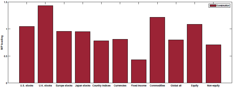
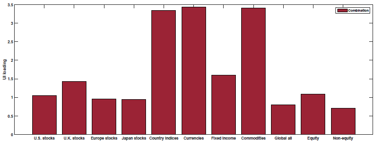
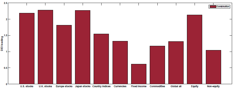
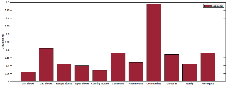
This is examined in Figure 4 of the paper (as well as Table 5). Below are the results with the red bar representing the loading on each macroeconomic factor for the 50/50 Value and Momentum portfolios:
Growth Rate of Industrial Production (MP)
Unexpected Inflation (UI)
Change in Expected Inflation (DEI)
Term Spread (UTS)
Default Spread (UPR)
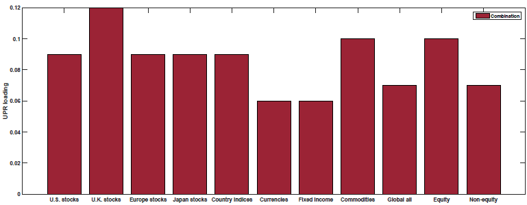
As shown above, the 50/50 Value and Momentum portfolios load positively on all of the macroeconomic risk factors.
Thus, the paper finds that (1) Value and Momentum portfolios load oppositely on five macroeconomic risk factors (giving insight to the negative correlation between the two) yet also showing that (2) the 50/50 combination loads positively on all the macroeconomic risk factors.
There is more in the paper, but to me, this paper was interesting in that it found a way to tie both Value and Momentum to macroeconomic risk factors.
However, this is still a working paper, which has not been updated for over a year. So what would some constructive criticism of the paper be? Well, luckily for me, this paper was presented at a 2017 conference. Here is a link to the video (also found below). In academic conferences, it is normal to have a discussant give the authors of the paper feedback/constructive criticism. This begins around the 38-minute mark of the video, by an FX expert, Nick Roussanov.(6)
Nick gives some comments on the paper which I summarize below (also found in the video!):
Nick comments:
- Success? Using 5 GRR factors has a lower GRS test statistic than the 3-factor model (as in the original AMP paper).
- One needs to be careful when using mimicking portfolios.
- Do we need all 5 factors? Nick shows that reducing the number of macroeconomic factors gives similar results.
- Nick shows that you can get similar results using 5 alternative factors, such as growth rates of the following 5 factors:(7)
- Assets of Commercial Banks
- Civilian Labor Force
- Passenger Car Registrations
- Loans and Leases in Bank Credit
- New Housing Permits
- Randomizing the weights on the mimicking portfolios yields the same GRS test statistic as the mimicking portfolios — so which factors are most important? (To be fair, the paper highlights that they do not address this in the paper).
Summary and Conclusion
So as Nick highlights (best understood by watching the video), the paper has some issues to be addressed. However, the paper shows that using their set of five macroeconomic factors, one finds that (1) Value and Momentum have opposite loadings on each macro factor and (2) the 50/50 Value and Momentum portfolio loads positively on the macro factors.
Let us know what you think …
Presentation of the Paper:
A Global Macroeconomic Risk Model for Value, Momentum, and Other Asset Classes
- Ilan Cooper, Andreea Mitrache, and Richard Priestley
- A version of the paper can be found here.
- Want a summary of academic papers with alpha? Check out our Academic Research Recap Category.
Abstract:
Value and momentum returns and combinations of them are explained by their loadings on global macroeconomic risk factors across both countries and asset classes. These loadings describe why value and momentum have positive return premia and why they are negatively correlated. The global macroeconomic risk factor model also performs well in summarizing the cross section of various additional asset classes. The findings identify the source of the common variation in expected returns across asset classes and countries suggesting that markets are integrated.

References[+]
| ↑1 | Hat tip to Lu Zhang’s 2013 article for pointing these quotes out |
|---|---|
| ↑2 | The details (for each asset class) can be found in the paper here. |
| ↑3 | Note, AMP ranks “all the securities, across markets and asset classes, by value and momentum and sort them into three equal groups. Thus, using the entire cross-section of securities, they generate three portfolios – low, middle, and high – for value and momentum, producing six well-diversified portfolios” |
| ↑4 | Created from the six AMP portfolios |
| ↑5 | But since we created the mimicking portfolios for the five macroeconomic risk factors from the six AMP portfolios, what is their relationship? The authors regress the mimicking portfolio on the AMP factor portfolios and find the adjusted R^2’s to be 0.16, 0.25, 0.26, 0.47, and 0.12–this gives us confidence that the factors are not merely different representations of the Value and Momentum factors. |
| ↑6 | Here is a podcast where Wes interviews Nick. |
| ↑7 | Note this required a Ph.D. student/Nick to generate the same results in the paper and then to generate new results using new macroeconomic factors! |
About the Author: Jack Vogel, PhD
—
Important Disclosures
For informational and educational purposes only and should not be construed as specific investment, accounting, legal, or tax advice. Certain information is deemed to be reliable, but its accuracy and completeness cannot be guaranteed. Third party information may become outdated or otherwise superseded without notice. Neither the Securities and Exchange Commission (SEC) nor any other federal or state agency has approved, determined the accuracy, or confirmed the adequacy of this article.
The views and opinions expressed herein are those of the author and do not necessarily reflect the views of Alpha Architect, its affiliates or its employees. Our full disclosures are available here. Definitions of common statistics used in our analysis are available here (towards the bottom).
Join thousands of other readers and subscribe to our blog.