A trend following strategy is based on switching between a financial asset and cash depending on whether the asset prices trend upward or downward. Specifically, when the strategy identifies that prices trend upward (downward), it generates a Buy (Sell) trading signal. A Buy signal is a signal to invest in the asset (or stay invested in the asset), whereas a Sell signal is, most common, a signal to sell the asset and invest in cash (or stay invested in cash). The other, less typical strategy, is to short the asset when a Sell signal is generated.
In this blog post we review the most common trend-following rules that are used by traders. Practically all of these rules are based on moving averages of prices. And in virtually all technical trading rules the generation of a trading signal is a two-step process. At the first step, the value of a technical trading indicator is computed using the past prices including the last closing price


where TR denotes the trading rule and f(.) denotes the function that specifies how the value of the technical trading indicator is computed. At the second step, the value of the technical indicator is translated into a trading signal. Typically, a Buy signal is generated when the value of the technical trading indicator is positive. Otherwise, a Sell signal is generated. That is,


Momentum Rule
We start with the Momentum (MOM) rule which seemingly has nothing to do with moving averages. However, in the subsequent blog post we show that this rule is inherently related to the rules based on moving averages. The Momentum rule represents the simplest and most basic market timing rule. In this rule, the last closing price Pt is compared with the closing price n-1 periods ago, Pt-n+1. A Buy signal is generated when the last closing price is greater than the closing price n-1 periods ago (in our notation, n denotes the size of the window used to compute a trading indicator). Implicitly, this rule assumes that if market prices have been increasing (decreasing) over the last n-1 periods, the prices will continue to increase (decrease) over the subsequent period. In other words, the n-1-period trend will continue in the future.
Formally, the technical trading indicator for the Momentum rule is computed as


The figure below, bottom panel, plots the values of the technical trading indicator of the MOM(12) rule computed using the monthly prices of the S&P 500 index over the period from January 1997 to December 2006. The top panel in this figure plots the values of the index. The shaded areas in this plot indicate the periods where this rule generates a Sell signal.
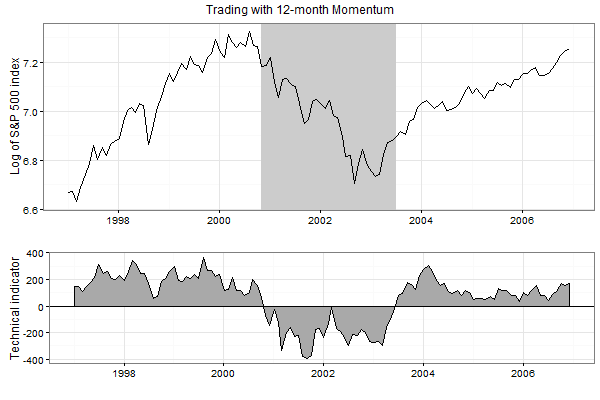
The results are hypothetical results and are NOT an indicator of future results and do NOT represent returns that any investor actually attained. Indexes are unmanaged, do not reflect management or trading fees, and one cannot invest directly in an index. Additional information regarding the construction of these results is available upon request.
The interactive illustration of trading with the Momentum rule can be found here.
Moving Average Change of Direction Rule
The idea behind this rule is based on a straightforward principle: if market prices are trending upward (downward), then the value of a moving average of prices tends to increase (decrease). In this rule, the most recent value of a moving average is compared with the value of this moving average in the preceding period. A Buy signal is generated if the value of a moving average has increased over the last period. Formally, the technical trading indicator for the Moving Average Change of Direction (ΔMA) rule is computed as


where MA(n) denotes a moving average of prices computed using the averaging window of size n.
The figure below, bottom panel, plots the values of the technical trading indicator of the ΔEMA(12) rule computed using the monthly prices of the S&P 500 index over the period from January 1997 to December 2006. The top panel in this figure plots the values of the index and the 12-month EMA. The shaded areas in this plot indicate the periods where this rule generates a Sell signal.
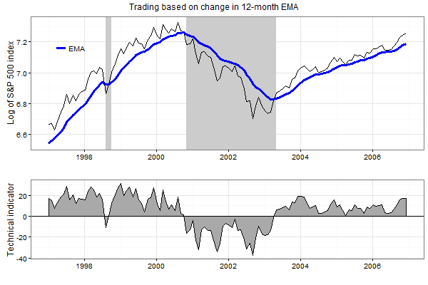
The results are hypothetical results and are NOT an indicator of future results and do NOT represent returns that any investor actually attained. Indexes are unmanaged, do not reflect management or trading fees, and one cannot invest directly in an index. Additional information regarding the construction of these results is available upon request.
The interactive illustration of trading with the Moving Average Change of Direction rule can be found here.
Price Minus Moving Average Rule
The Price Minus Moving Average (P-MA) rule is the oldest and one of the most popular trading rules that use moving averages. The principle behind this rule is based on the lagging property of a moving average. Specifically, in Part 1 we showed explicitly that, when stock prices are trending upward, the moving average lies below the price. In contrast, when stock prices are trending downward, the moving average lies above the price. Therefore, to identify the direction of the trend, in this rule the last closing price is compared with the value of a moving average. A Buy signal is generated when the last closing price is above the moving average. Otherwise, if the last closing price is below the moving average, a Sell signal is generated. Formally, the technical trading indicator for the P-MA rule is computed as


The figure below, bottom panel, plots the values of the technical trading indicator of the P-SMA(10) rule computed using the monthly prices of the S&P 500 index over the period from January 1997 to December 2006. The top panel in this figure plots the values of the index and the values of the 10-month SMA. The shaded areas in this plot indicate the periods where this rule generates a Sell signal.
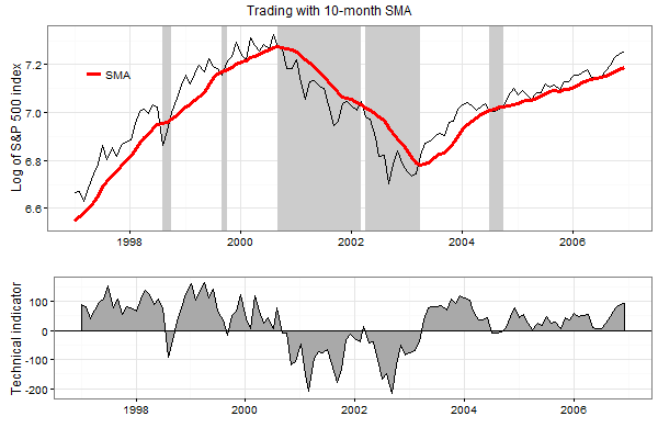
The results are hypothetical results and are NOT an indicator of future results and do NOT represent returns that any investor actually attained. Indexes are unmanaged, do not reflect management or trading fees, and one cannot invest directly in an index. Additional information regarding the construction of these results is available upon request.
The interactive illustration of trading with the Price Minus Moving Average rule can be found here.
Moving Average Crossover Rule
Because the price is noisy, the Price Minus Moving Average rule produces many false signals. This issue is especially relevant when prices trend sideways or when trading happens at the daily frequency. One of several remedies that allow a trader to reduce the number of whipsaw trades is to employ two moving averages in the generation of a trading signal: one shorter average with window size of s and one longer average with window size of l>s. This technique is called the Moving Average Crossover (MAC) rule. In this case the technical trading indicator is computed as


A crossover occurs when a shorter moving average crosses either above or below a longer moving average. The former crossover is usually dubbed as a bullish crossover or a “golden cross”. The latter crossover is usually dubbed as a bearish crossover or a “death cross”. The most typical combination in daily trading is to use two SMAs with window sizes of 50 and 200 days. Other types of moving averages can also be used in the MAC rule.
The figure below, bottom panel, plots the values of the technical trading indicator of the MAC(3,10) rule computed using the monthly prices of the S&P 500 index over the period from January 1997 to December 2006. The top panel in this figure plots the values of the index and the values of 3- and 10-month SMAs. The shaded areas in this plot indicate the periods where this rule generates a Sell signal. It is instructive to compare the number of Sell signals in the P-SMA(10) rule (illustrated in the figure above) with the number of Sell signals in the MAC(3,10) rule: whereas over the 10-year period 1997-2006 the P-SMA(10) rule generated 5 Sell signals, the MAC(3,10) rule generated only 3 Sell signals.

The results are hypothetical results and are NOT an indicator of future results and do NOT represent returns that any investor actually attained. Indexes are unmanaged, do not reflect management or trading fees, and one cannot invest directly in an index. Additional information regarding the construction of these results is available upon request.
The interactive illustration of trading with the Moving Average Crossover can be found here.
Moving Average Envelope
The other possibility to reduce the number of false trading signals is to use a Moving Average Envelope (MAE). Specifically, a moving average envelope consists of two boundaries above and below a moving average. The distance from the moving average and a boundary of the envelope is usually specified as a percentage (for example, 5%). As long as the price lies within these two boundaries, no trading takes place. A Buy (Sell) signal is generated when the price increases above (decreases below) the upper (lower) boundary of the envelope. Formally, denote by MAt(n) the moving average of prices over a window of size n and by p the envelope percentage. The lower (L) and upper (U) boundaries of the moving average envelope are computed as


Mathematically, the trading signal is generated according to:


The figure below plots the values of the S&P 500 index over the period from January 1997 to December 2006, as well as the values of the upper and lower boundaries of the moving average envelope. The shaded areas in this plot indicate the periods where this rule generates a Sell signal. Whereas over the 10-year period 1997-2006 the P-SMA(10) rule generated 5 Sell signals, the MAE(10,5) rule generated only 2 Sell signals.
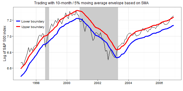
The results are hypothetical results and are NOT an indicator of future results and do NOT represent returns that any investor actually attained. Indexes are unmanaged, do not reflect management or trading fees, and one cannot invest directly in an index. Additional information regarding the construction of these results is available upon request.
The interactive illustration of trading with the Moving Average Envelope can be found here.
Moving Average Convergence/Divergence Rule
A different approach to the generation of a trading signal is suggested by Gerald Appel. Specifically, he proposed the Moving Average Convergence/Divergence (MACD) rule which is a combination of three EMAs. The first step in this rule is to compute the regular MAC indicator using two EMAs


Recall that in the regular MAC rule a Buy signal is generated when the shorter moving average is above the longer moving average. In the late 1970s, Gerald Appel suggested to generate a Buy (Sell) signal when MAC increases (decreases). Specifically, in this case a Buy (Sell) signal is generated when the shorter moving average increases (decreases) faster than the longer moving average. In order to reduce the number of false signals, Gerald Appel suggested additionally that a directional movement in MAC must be confirmed by a delayed and smoothed version of MAC. As a result, in the MACD rule the technical trading indicator is computed as


The principle behind the computation of the trading indicator of the MACD rule is the same as that in the Price Minus Moving Average rule. In particular, if MAC is trending upward (downward), a moving average of MAC tends to be below (above) MAC.
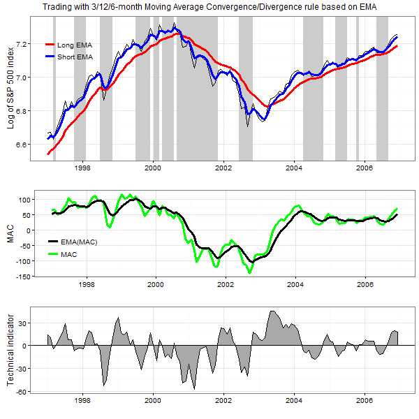
The figure below, bottom panel, plots the values of the technical trading indicator of the MACD(3,12,6) rule computed using the monthly prices of the S&P 500 index over the period from January 1997 to December 2006. The top panel in this figure plots the values of the index as well as the values of 3- and 12-month EMAs. The shaded areas in this plot indicate the periods where this rule generates a Sell signal. The middle panel in this figure plots the values of the MAC(3,12) and the EMA(6,MAC(3,12)).
The results are hypothetical results and are NOT an indicator of future results and do NOT represent returns that any investor actually attained. Indexes are unmanaged, do not reflect management or trading fees, and one cannot invest directly in an index. Additional information regarding the construction of these results is available upon request.
It is worth noting that the MACD rule, as its name suggests, is devised to generate trading signals when the two moving averages in the MAC indicator either converge or diverge. As a result, the trading signals are generated when the trend either strengthens or weakens. For example, when the price moves upward with an increasing speed, the shorter moving average increases faster than the longer moving average. If the shorter moving average is located above (below) the longer moving average, the two moving averages diverge (converge). Because the value of the MAC increases, the MACD rule generates a Buy signal regardless of the location of the shorter moving average relative to the location of the longer moving average.
Last but not least, it is important to emphasize that, since the MACD rule is devised to react to the changes in the price trend, the MACD rule is most suited when the price trend often changes its direction (that is, when prices are mean-reverting). In contrast, when prices trend steadily, both the moving averages move parallel. In this case even small changes in the price dynamics are able to generate lots of false trading signals.
The interactive illustration of trading with the Convergence/Divergence rule can be found here.
Summary
The success of a trend following strategy depends on its ability to timely identify the direction of the trend in prices. However, fluctuations in prices make it difficult to recognize the direction of the price trend. Moving averages are often used to smooth these fluctuations in order to highlight the underlying trend.
Even though the concept of trend following is simple (“jump on a trend and ride it”), there is no unique practical realization of a trend following strategy. There are trend following rules that do not employ moving averages. There are trend following rules that use only one moving average. But even in this case, there are two possible methods of generation of a Buy signal: either when the value of a moving average increases, or when the value of a moving average lies below the price. In addition, there are trend following rules that employ two, three, and even multiple moving averages. As a rule, the supplementary moving averages are used to improve the performance of a moving average trading strategy.
When prices trend steadily upward or downward, moving averages easily identify the direction of the trend. In these cases, all moving average trading rules generate correct Buy and Sell trading signals, albeit with some delay. However, when prices trend sideways, moving average rules tend to generate many false signals, otherwise known as “whipsaws”. These whipsaw trades are unnecessary trades that deteriorate the profitability of a trading strategy. There are a few remedies that allow a trader to reduce the number of whipsaw trades.
The moving average trading strategies are advantageous when the trend is strong and long-lasting. However, the advantages of the moving average strategies may disappear completely when the trend is weak. Due to the lagging nature of any moving average, the advantages of the moving average strategies may disappear even if the trend is strong but short-lasting. Unfortunately, no remedy exists to deal with the lagging property of a moving average. It is worth noting that all techniques that reduce the number of whipsaw trades usually achieve that at the expense of increasing the delay in turning point identification.
Where to learn more?
You can read the entire series here.
Editor’s Note
I am an idiot and sent out #4 last week. This installment is #3. Next week we’ll have #5. Sorry for the confusion.
About the Author: Valeriy Zakamulin
—
Important Disclosures
For informational and educational purposes only and should not be construed as specific investment, accounting, legal, or tax advice. Certain information is deemed to be reliable, but its accuracy and completeness cannot be guaranteed. Third party information may become outdated or otherwise superseded without notice. Neither the Securities and Exchange Commission (SEC) nor any other federal or state agency has approved, determined the accuracy, or confirmed the adequacy of this article.
The views and opinions expressed herein are those of the author and do not necessarily reflect the views of Alpha Architect, its affiliates or its employees. Our full disclosures are available here. Definitions of common statistics used in our analysis are available here (towards the bottom).
Join thousands of other readers and subscribe to our blog.