Shiller’s CAPE ratio is a popular and useful metric for measuring whether stock prices are overvalued or undervalued relative to earnings. Recently, Vanguard analysts Haifeng Wang, Harshdeep Singh Ahluwalia, Roger A. Aliaga-Díaz, and Joseph H. Davis have written a very interesting paper on forecasting equity returns using Shiller’s CAPE and machine learning: “The Best of Both Worlds: Forecasting US Equity Market Returns using a Hybrid Machine Learning – Time Series Approach“.
First, what is the Shiller CAPE ratio?(1)
To calculate it we need the following:
- Take 10 years of trailing earnings
- Compute real earnings by adjusting the earnings for inflation to the current CPI price level
- Divide the current market cap of the stock (or index) by average annual real earnings
If we do a simple regression of Shiller’s CAPE ratio against future 10-year returns, we observe a very strong relationship.
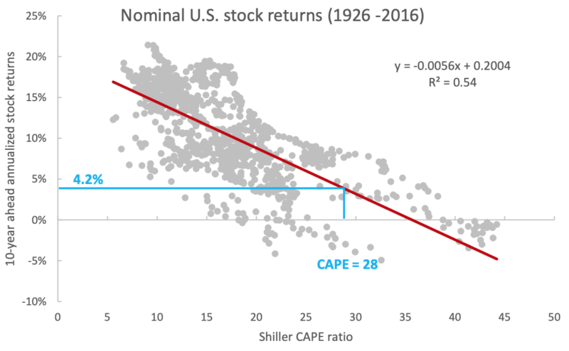
Here we see a historical chart of actual 10-year annualized stock returns vs. those predicted by Shiller’s CAPE. Using the Shiller regression, the current CAPE of about 30 suggests near-zero real return over the next 10 years.
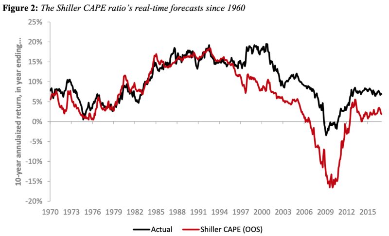
These charts are from the noteworthy 2018 paper “Improving U.S. stock return forecasts: A “fair-value” CAPE approach” by Vanguard analysts Joseph H. Davis, Roger Aliaga-Díaz, Harshdeep Ahluwalia, and Ravi Tolani, previously discussed on Alpha Architect here. The first three authors also co-authored the 2019 machine learning paper.
As the authors discussed, the CAPE ratio has produced a worsening forecasting record in recent years. Since 1985, forecasts based on the Shiller CAPE regression have generated an RMSE of about 7.8%. That’s a large error in an annual return forecast, and forecasts have been consistently too low, as the CAPE has remained persistently high relative to its long-term average.
One criticism of CAPE is that reductions in real interest rates, if persistent, justify a higher P/E. Another is that changes in accounting standards and payouts v. buybacks require adjusting the CAPE model for consistency over time. Jeremy Siegel created a reformulated CAPE which uses NIPA earnings instead of reported earnings.
Which brings us to the recent paper. First, the authors used a machine-learning approach to the original Shiller regression. Instead of the simple univariate regression, they added additional variables, tuned several machine learning models, and ensembled them.
The model form is as follows:

where
- CAPE is the cyclically adjusted price/earnings (P/E) ratio
- Y is Real 10-year bond yields, or nominal Treasury yield less an estimated 10-year expected inflation rate
- CPI is Year-over-year CPI inflation rate
- SPVol is the Realized S&P500 price volatility, over trailing 12 months
- BondVol is the Realized volatility of changes in our real bond yield series, over trailing 12 months
- SVAR is the stock variance computed as sum of squared daily returns on S&P 500
- TBL is the treasure bill rates
- DFY is the default yield spread computed as the difference between BAA- and AAArated corporate bond yields
- DFR is the default return spread, computed as the difference between the return on longterm corporate bonds and returns on the long-term government bonds
The CAPE response is modeled using these 8 predictors and 4 machine learning regression algorithms: Random Forest, Gradient Boost, Support Vector Machine and Gated Recurrent Unit (a form of recurrent neural network). Hyperparameters are chosen using time-based cross-validation, starting with the 1926-1959 period and walking forward one month at a time, and choosing the best-performing hyperparameters in the cross-validation set.
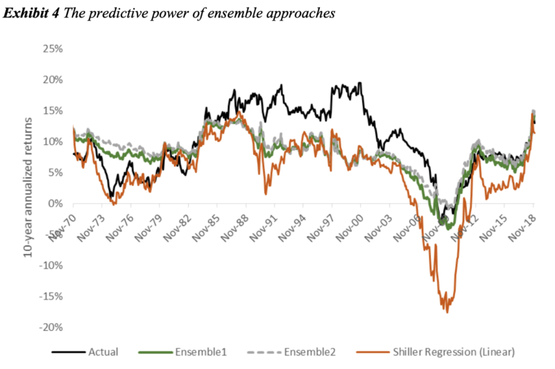
Individual ML algorithms displayed small to no advantage vs. the linear regression. An ensemble equal-weighting all the ML models obtained a noteworthy improvement in RMSE vs. a linear regression (4.7% RMSE vs 6.6%). GBM performed best. Boosting algorithms, such as XGBoost and LightGBM, are currently considered state-of-the-art for plain-vanilla tabular forecasting, as opposed to deep learning. While ensembling several algorithms increases the complexity of the forecasting process, it results in more accurate and robust predictions; Kaggle contests are generally won by ensembles, not single-algorithm forecasts.
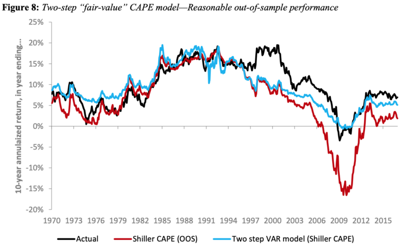
In a second machine learning experiment, the authors applied a 2-step forecasting process pioneered in the Vanguard 2018 paper, enhanced with machine learning.
In the 2018 Vanguard paper, a linear vector autoregression (VAR) was used. In the first step, the fair-value CAPE was estimated using a VAR model of five variables. Each month, each variable is modeled as a linear function of the values of these five variables for the 12 preceding months:
- CAPE real earnings yield, or 1/CAPE
- Real 10-year bond yields, or nominal Treasury yield less an estimated 10-year expected inflation rate
- Year-over-year CPI inflation rate
- Realized S&P 500 price volatility, over trailing 12 months
- Realized volatility of changes in a real bond yield series, over trailing 12 months.
The model can then be used to forecast a value the CAPE is expected to revert to over 10 years under VAR dynamics, such that the long-run CAPE is consistent with long-run relationships between the variables, and also recent levels of those variables.
In the second step, the authors back out the nominal (or real) equity market return implied by the CAPE forecast.
In the 2018 paper, the analysts found a notable improvement in the forecast using a linear VAR version of this methodology.
In the latest 2019 paper, the same 2-step process is used, but machine learning models are used instead of linear VAR.
Again, each machine learning model is tuned using walk-forward cross-validation to optimize the bias-variance tradeoff for best performance, and the models are ensembled.
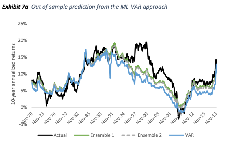
A better forecast (2.6% RMSE) was obtained vs. the linear VAR (3.8% RMSE), which in turn was significantly superior to a linear Shiller regression (6.6% RMSE).
By any measure, the current CAPE of over 30 is elevated and points to sub-par future returns, but the more complex models point to moderate returns as opposed to near-zero real returns.
Conclusion
This paper is a great example of applying machine learning to improve forecasting. Machine learning tends to need a lot of data, but even on monthly data, we see a potentially useful result.
Machine learning is a highly empirical paradigm with no priors on the functional form. Instead of assuming a linear relationship, we can allow the algorithm to find a highly nonlinear model.
In any scientific endeavor, there is a tension between theory and experiment. If you don’t check a theory against real-world data, it’s unlikely to be very good. But if all you do is predict according to past data, without deep theoretical understanding, then as soon as you encounter a future unlike the past, your model is likely to fail.
Machine learning leans toward the latter approach, in that it does not have a strong prior on the functional form of the model relationships. Machine learning models can be sensitive to small departures from past experience. Sometimes the result is a brittle model, for instance, vulnerability to adversarial attacks. In this context of financial modeling, if we get data we haven’t seen in the past, e.g. negative rates, it’s hard to say what the forecast dynamics are going to be using machine learning to forecast the CAPE. Additionally, the complexity of machine learning models can make them hard to interpret.
I like to say that machine learning is statistics for street-fighting. With simple linear models, sometimes you don’t get great results, but you know why: your model doesn’t capture everything, and your data doesn’t perfectly fit the assumptions of normality, etc. With machine learning, sometimes you get better results, but you’re not always sure why: it can be hard to understand exactly what the model is doing.
If you have good data, machine learning forecasting usually just works better in practice. And this paper is a great example of using machine learning models to improve outcomes on a finance problem with important practical implications.
References[+]
| ↑1 | Here is a post. |
|---|
About the Author: Druce Vertes
—
Important Disclosures
For informational and educational purposes only and should not be construed as specific investment, accounting, legal, or tax advice. Certain information is deemed to be reliable, but its accuracy and completeness cannot be guaranteed. Third party information may become outdated or otherwise superseded without notice. Neither the Securities and Exchange Commission (SEC) nor any other federal or state agency has approved, determined the accuracy, or confirmed the adequacy of this article.
The views and opinions expressed herein are those of the author and do not necessarily reflect the views of Alpha Architect, its affiliates or its employees. Our full disclosures are available here. Definitions of common statistics used in our analysis are available here (towards the bottom).
Join thousands of other readers and subscribe to our blog.