Timing Value and Momentum with Valuation-Spreads -

We were recently passed along an article suggesting that valuation spreads, or the spread in a valuation metric across the most expensive and least expensive stocks, matters for timing investments.

We take this concept one step further and investigate if valuation spreads can help us time value and momentum exposures. We hypothesize that if there are large spreads in valuation across the cheapest stocks and the most expensive stocks, this may indicate a value premium (“stock picker’s market”), while a small valuation spread may indicate a momentum premium (“a trending market”).

Of course, a natural reaction is — wow — investors should definitely seek to time their allocations to value investing funds and momentum investing funds based on the “value spread” timing indicator.

Sounds like a great story. Let’s see what the evidence suggests.

Sadly, as is often the case in investing, the story sounds a lot better than the results.

We find little evidence that valuation-spreads can time value and momentum.

Background

You’ve probably heard the statistics joke: your head is in the oven and your feet are in the fridge, on average you’re 72 degrees and life is great. Of course, you are also dead, and averages have managed to confuse us more than help us–a common flaw of statistical averages.

An analogous flaw of “averages” could be made in the context of financial markets. If the “average” P/E on the market is in the 99th percentile, then “of course,” you should not be invested. We debunked this concept a few days ago.

But perhaps valuation-based timers can be useful, but we just need to dig a little deeper?

The problem with averages is they can’t communicate the “tails” of a distribution.

Take 2 scenarios, each with an average P/E of 50:

Scenario 1: 3 stocks in the universe: A, B, and C. PE_A=1, PE_B=50, and PE_C=99. The average P/E is 50, or in the 99th percentile of history.
Scenario 2: 3 stocks in the universe: A, B, and C. PE_A=49, PE_B=50, and PE_C=51. The average P/E is 50, or in the 99th percentile of history.

In scenario 1, there might be an amazing opportunity in the marketplace: stock A is selling at a PE of 1! With scenario 2, we might be more inclined to fear the market since all stocks are expensive. There are other scenarios one can draw up, which highlight the utter uselessness of averages. For example, imagine we witness a high market average PE of 35, but this PE is heavily skewed by a handful of mega-cap social media companies with PEs of 200+. What this high market average PE doesn’t tell us is that the other 95% of companies have a PE of 5!

As illustrated above, by simply looking at average market valuations we miss some important information. Averages don’t tell us much, on average (a bad statistics joke, sorry).

Perhaps we can glean useful information from valuations, by examining the ‘tails’ of the distribution?

Building a Valuation-Spread Timing Mechanism

To create our “valuation-spread variable” we do the following:
Step 1: Sort stocks from the sample period into 10 deciles based on EBIT/TEV (we only focus on US mid/large cap to avoid weird micro/small cap outlier effects)

Let’s say we have 1,000 stocks in the universe. We can calculate the EBIT/TEV for all stocks in the universe. We can then divvy the stocks into buckets–say, 10 deciles, or 100 stocks in each bucket.

Step 2: Calculate the EBIT yield spread of each month= (average EBIT for the top 10% cheap) – (average EBIT for the bottom 10% expensive)

Cheap EBIT/TEV decile has an average yield of 15%; expensive decile has an average yield of 5% ==> Value spread = 10%

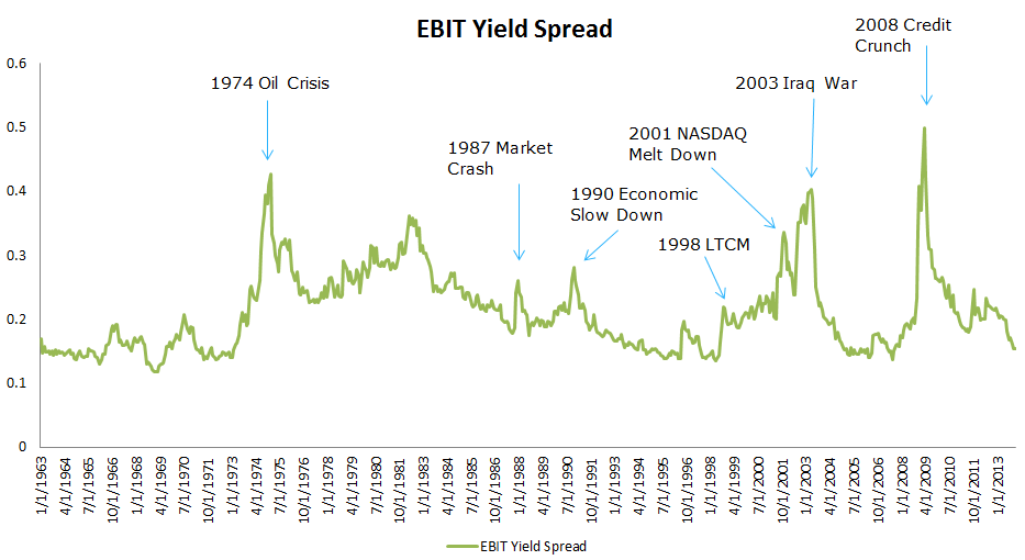
The graph below shows the Valuation Spreads from 1/1963 to 12/2013. We highlighted spikes for associated stress events.

The results are hypothetical results and are NOT an indicator of future results and do NOT represent returns that any investor actually attained. Indexes are unmanaged, do not reflect management or trading fees, and one cannot invest directly in an index. Additional information regarding the construction of these results is available upon request.

We use valuation spreads to time value and momentum using various lookback periods, such as 3 months, 12 months, and 120 months. Here is an example of how we use the valuation spreads:

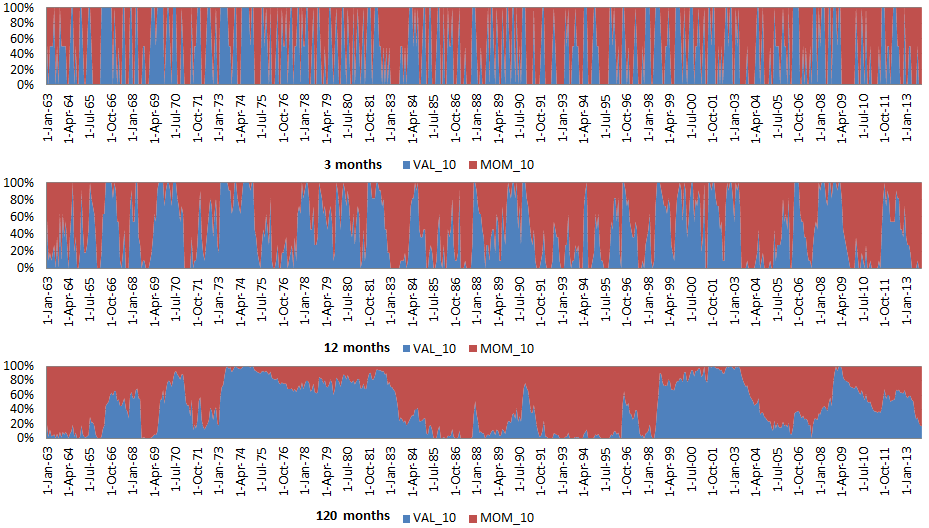
Looking back 3 months, the weight on value at time 0 is the percentile rank of the EBIT Yield Spread at T-1 over the last 3 months (T-1 to T-3); the weight of momentum is 1 minus the weights of value.

Note how our model dynamically allocates to value and momentum, based on how wide, or narrow the spread is. That is, we allocate more to one, when spreads are wide in it, and less when spreads are narrow.

Data Details

Our historical data period is from 1/1/1963 to 12/31/2013. For our portfolios, we use Fama-French value top decile (VAL_10) and momentum top decile (MOM_10) as underlying portfolios (value-weight returns).

Benchmark returns are gross of fees, constructed portfolios (marked with a “net”) are net of a 1% annual fee. All returns are total returns and include the reinvestment of distributions (e.g., dividends).

Here is the legend for the portfolios and benchmarks analyzed:

50/50 VAL MOM (net) = 50% in VAL_10 and 50% in MOM_10
VAL_10 = Ken French Top Decile Value (Value-weighted portfolio). Click here to get data.
MOM_10 = Ken French Top Decile Momentum (Value-weighted portfolio). Click here to get data.
SP500 = S&P 500 Total Return Index
VAL_MOM_3M EBIT (net) = Weight in VAL_10 is the percentile of EBIT yield spread relative to the last 3 months, and the weight in MOM_10 is 1 minus the VAL_10 weight.
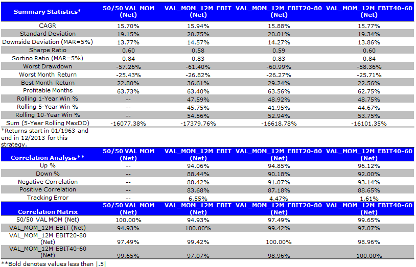
VAL_MOM_12M EBIT (net) = Weight in VAL_10 is the percentile of EBIT yield spread relative to the last 12 months, and the weight in MOM_10 is 1 minus the VAL_10 weight.
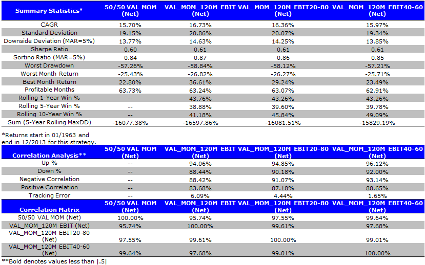
VAL_MOM_120M EBIT (net) = Weight in VAL_10 is the percentile of EBIT yield spread relative to the last 120 months, and the weight in MOM_10 is 1 minus the VAL_10 weight.

Benchmark Summary Statistics

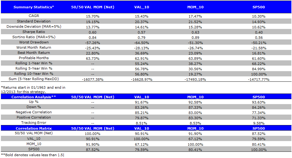
Before we undertake our spread-based analysis, we want to review how these strategies perform in a static environment (i.e., no timing based on spreads). We first review some stats for value and momentum portfolios, as well as a combination portfolio that has 50% value and 50% momentum (monthly-rebalanced back to 50/50). The time period is from 1/1/1963 to 12/31/2013. Also, as a point of clarification, we added a 1% management fee on the proposed 50/50 value/momentum blend, since this is a constructed strategy.

Summary Statistics:

VAL_10 and MOM_10 outperform the SP500.
The 50/50 strategy improves risk-adjusted performance.

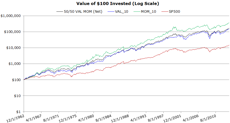
Invested Growth

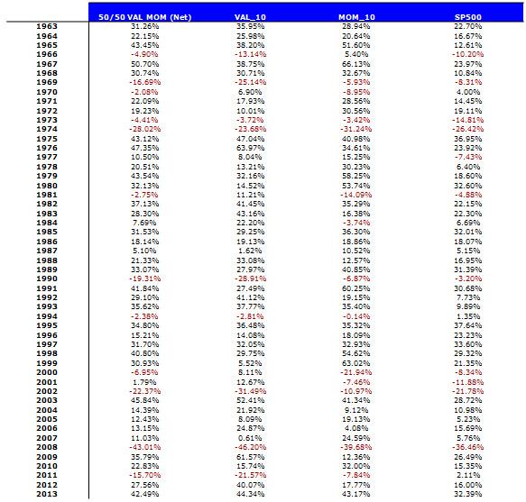
Annual Returns

Valuation-Spread Timing Summary Statistics

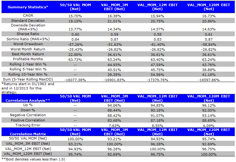
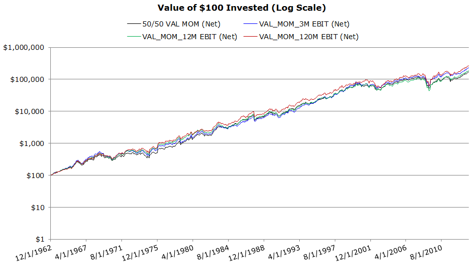
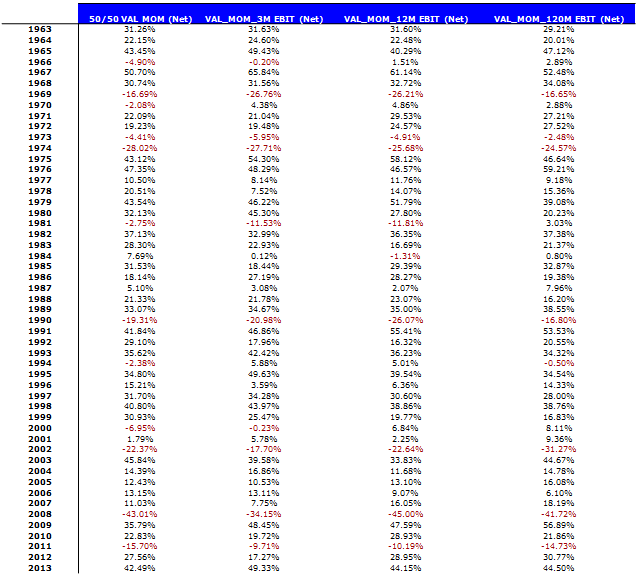
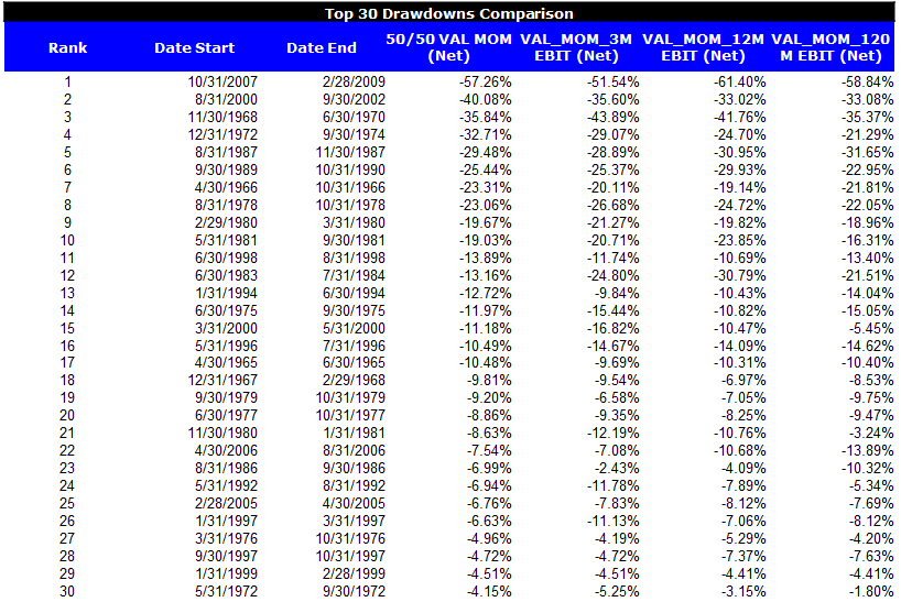
Now for the heart of the analysis. In this section, we investigate whether using valuation-spread indicators to shift weights between value and momentum improve upon a simple 50/50 value/momentum portfolio. The valuation-spread indicators are assessed monthly. The time period is from 1/1/1963 to 12/31/2013. We add a 1% management fee on all four constructed strategies. All return are total returns and include the reinvestment of distributions (e.g., dividends).

Summary Statistics

The 50/50 val/mom equal-weight benchmark performs similarly to the timing methods.

Nothing obvious is jumping out at us yet.

Invested Growth

Annual Returns

Top Drawdowns

Time Series of Val/Mom Weights

Here we investigate the weights in value and momentum from month to month from 1/1/1963 to 12/31/2013.

Shorter look-back periods generate more transactions, and thus, would be more expensive to implement in a real-world scenario.

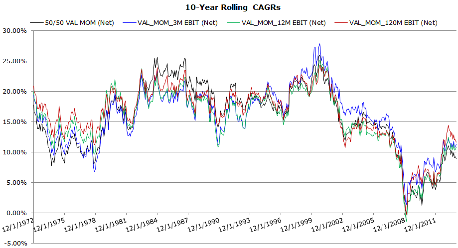
Robustness Analysis — Rolling CAGRs

Results are similar to the 50/50 strategy

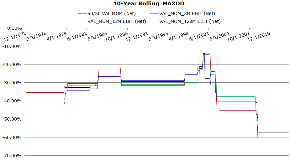
Robustness Analysis — Rolling MAXDD

More Sophisticated Valuation-Spread Timing Models

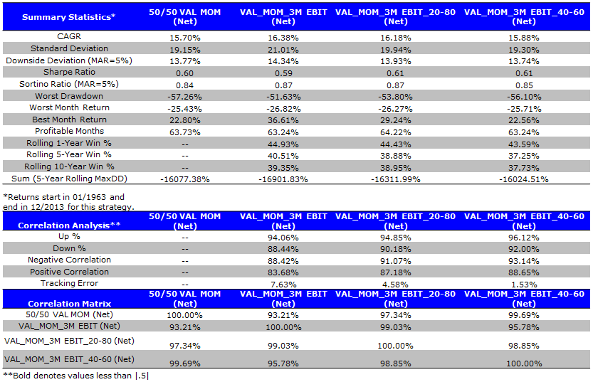
To decrease transaction frequency we test truncated weighting schemes. For instance, in our 20-80 system, the weights have a lower limit of 20% and a upper limit of 80%. That is, if the model indicates a 15% value allocation, we will allocate 20% in value; if model says 85% in value, we will allocate 80% in value. This simple refinement prevents the model signal from wildly swinging allocations between value and momentum.

Our historical data period is still from 1/1/1963 to 12/31/2013. Here are the portfolios:

50/50 VAL MOM (net) = 50% in VAL_10 and 50% in MOM_10
VAL_MOM_3M EBIT (net) = Weight in VAL_10 is the percentile of EBIT yield spread in last 3 months, and weight in MOM_10 is 1 minus the percentile.
VAL_MOM_3M EBIT_20-80 (net) = Weight in VAL_10 is the percentile of EBIT yield spread in last 3 months, and weight in MOM_10 is 1 minus the percentile. The weightings have a lower limit of 20% and a upper limit of 80%. For example, if model says 15% in value, then we will allocate 20% in value; if model says 85% in value, we will allocate 80% in value.
VAL_MOM_3M EBIT_40-60 (net) = Weight in VAL_10 is the percentile of EBIT yield spread in last 3 months, and weight in MOM_10 is 1 minus the percentile. The weightings have a lower limit of 40% and a upper limit of 60%. For example, if model says 15% in value, then we will allocate 40% in value; if model says 85% in value, we will allocate 60% in value.

All return are net, with 1% annual fees applied. All return are total returns and include the reinvestment of distributions (e.g., dividends).

Summary Statistics–3-month look-back

Results are similar to the 50/50 strategy

Summary Statistics–12-month look-back

Results are similar to the 50/50 strategy

Summary Statistics–120-month look-back

Results are similar to the 50/50 strategy

Conclusion

Overall, the timing model has higher annual returns, but it does not perform better on a risk-adjusted basis (Sharpe and Sortino ratios). This analysis is done with a 1% annual fee but the trading costs associated with switching between value and momentum and constructing the underlying portfolios could be more substantial.

The results suggest that a simple 50/50 allocation works just as well–if not better–than more sophisticated allocation systems.

Important Note: Yang Xu cranked a lot of numbers to make this post happen!

About the Author: Wesley Gray, PhD

After serving as a Captain in the United States Marine Corps, Dr. Gray earned an MBA and a PhD in finance from the University of Chicago where he studied under Nobel Prize Winner Eugene Fama. Next, Wes took an academic job in his wife’s hometown of Philadelphia and worked as a finance professor at Drexel University. Dr. Gray’s interest in bridging the research gap between academia and industry led him to found Alpha Architect, an asset management firm dedicated to an impact mission of empowering investors through education. He is a contributor to multiple industry publications and regularly speaks to professional investor groups across the country. Wes has published multiple academic papers and four books, including Embedded (Naval Institute Press, 2009), Quantitative Value (Wiley, 2012), DIY Financial Advisor (Wiley, 2015), and Quantitative Momentum (Wiley, 2016). Dr. Gray currently resides in Palmas Del Mar Puerto Rico with his wife and three children. He recently finished the Leadville 100 ultramarathon race and promises to make better life decisions in the future.

—

Important Disclosures

For informational and educational purposes only and should not be construed as specific investment, accounting, legal, or tax advice. Certain information is deemed to be reliable, but its accuracy and completeness cannot be guaranteed. Third party information may become outdated or otherwise superseded without notice. Neither the Securities and Exchange Commission (SEC) nor any other federal or state agency has approved, determined the accuracy, or confirmed the adequacy of this article.

The views and opinions expressed herein are those of the author and do not necessarily reflect the views of Alpha Architect, its affiliates or its employees. Our full disclosures are available here. Definitions of common statistics used in our analysis are available here (towards the bottom).

Join thousands of other readers and subscribe to our blog.

Background

Building a Valuation-Spread Timing Mechanism

Data Details

Benchmark Summary Statistics

Summary Statistics:

Invested Growth

Annual Returns

Valuation-Spread Timing Summary Statistics

Summary Statistics

Invested Growth

Annual Returns

Top Drawdowns

Time Series of Val/Mom Weights

Robustness Analysis — Rolling CAGRs

Robustness Analysis — Rolling MAXDD

More Sophisticated Valuation-Spread Timing Models

Summary Statistics–3-month look-back

Summary Statistics–12-month look-back

Summary Statistics–120-month look-back

Conclusion

About the Author: Wesley Gray, PhD

Important Disclosures

Are You Ready to Become a Better Investor?

Get Updates Now

Recent Posts

Important Disclosures