Tian, the newest team member, did a nice study on the “Sell in May and Go Away” phenomenon.
It has been an old axiom in stock market for generations: Sell in May and Go Away. Many readers may have heard of it. The idea is that the summer is a bad time to invest; fall/winter/spring are better.
Today is the first day of May, should we consider selling our stocks and go to cash?
Does this strategy actually work?
“Sell in May and Go Away” is also known as the Halloween indicator, which suggests that we sell stocks in May and buy again in November, especially around Halloween. Bouman and Jocobsen (2002) finds that the ‘Sell in May’ effect outperforms in 36 of 37 developed and emerging markets. They do further out-of-sample test by expanding their sample time horizon to 319 years and also applying their methodology to 108 markets across the world in their 2012 paper. They find that the effect holds even over this period. During the November-April period, when you are supposed to be in the market, returns are 6.25% higher than the May-October period, representing the Sell in May and Go Away period; the effect has persisted over the past 50 years. Moreover, this strong market anomaly has actually strengthened, rather than weakened, in recent years. Also, this effect is prevailing and statistically significant everywhere and all the time!
Wes and the team have done similar tests on international markets, but today we are going to focus on mainstream equity, alternative, and bond asset classes.
Our test assets include:
- Stocks:
- VW_CRSP: value-weighted CRSP index, 1927/1-2014/3
- EW_CRSP: equal-weighted CRSP index, 1927/1-2012/12
- SP500: S&P 500 Total Return index, 1927/1-2014/3
- SP500 EW: equal-weighted Total Return S&P 500 index, 1963/1-2014/3
- R2K: Russell 2000 Total Return index, 1979/1-2014/3
- EAFE: MSCI EAFE Total Return Index, 1975/2-2014/3
- EEM: MSCI Emerging Markets Total Return Index, 1975/2-2014/3
- Alternatives:
- REIT: FTSE NAREIT All Equity REITS Total Return Index , 1975/2-2014/3
- GSCI: S&P GSCI, 1975/2-2014/3
- SMB: Size factor, 1927/1-2014/2
- HML: Value factor, 1927/1-2014/2
- MOM: Momentum factor, 1927/1-2014/2
- Bonds:
- LTR: 10-Year Total Return Index, 1927/1-2014/3
- Source: Bloomberg and Ken French website
What do the results look like?
Let’s first take a look at the market performances during November- April (winter returns) period and May-October (summer returns) period based on 13 different asset indexes, with a time horizon of 87 years. Figure 1 shows the annualized returns based on two different strategies. Blue columns represent “sell in May” strategy, which is to sell stocks in early May and turn to T-bill markets, and then buy back around November. The opposite strategy is to buy stocks in May and sell in early November. The results show that November-April period returns substantially outperform the May-October period returns, with an average difference of 8.22% in equity markets, and 3.42% in alternative markets. Only the bond market shows insignificantly underperformance of “sell in May strategy” (-0.73%). Such strong overall performance, especially in stock markets, indicates that “Sell in May strategy” is worth digging into a little more deeply.
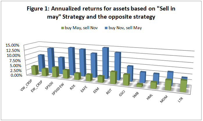
The results are hypothetical results and are NOT an indicator of future results and do NOT represent returns that any investor actually attained. Indexes are unmanaged, do not reflect management or trading fees, and one cannot invest directly in an index. Additional information regarding the construction of these results is available upon request.
To take a more careful look at how the “Sell in May strategy” beat the “Buy-and-Hold strategy,” as well as the “Buy May, sell Nov Strategy”, Figure 2 shows how an initial investment of $1,000,000 grows during the last 34 years (Russell 2000 index serves as the asset class). Clearly, the “Sell in May and go away” strategy has performed admirably, at least historically.
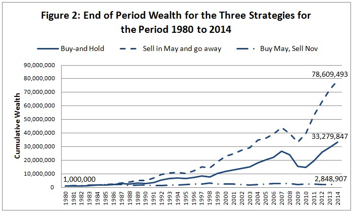
The results are hypothetical results and are NOT an indicator of future results and do NOT represent returns that any investor actually attained. Indexes are unmanaged, do not reflect management or trading fees, and one cannot invest directly in an index. Additional information regarding the construction of these results is available upon request.
The evidence in Figure 1 suggests that the Halloween effect is prominent among different assets, especially in stock markets. Another way to examine these results is via a month-to-month Sharpe Ratio analysis. Sharpe Ratios during the November- April (winter) period are much greater than those during May-October (summer) period. Moreover, among the 156 months associated with the 13 asset class samples (13*12=156), negative Sharpe ratios occurs 33 times, and 26/33 (around 80%) of these negative Sharpes occur during the May-October period. But as we can see below, the performance of the strategy depends on the asset class analyzed.
SP 500–marginal
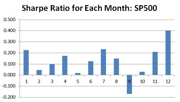
The results are hypothetical results and are NOT an indicator of future results and do NOT represent returns that any investor actually attained. Indexes are unmanaged, do not reflect management or trading fees, and one cannot invest directly in an index. Additional information regarding the construction of these results is available upon request.
LTR–terrible

The results are hypothetical results and are NOT an indicator of future results and do NOT represent returns that any investor actually attained. Indexes are unmanaged, do not reflect management or trading fees, and one cannot invest directly in an index. Additional information regarding the construction of these results is available upon request.
SP 500 EW–great
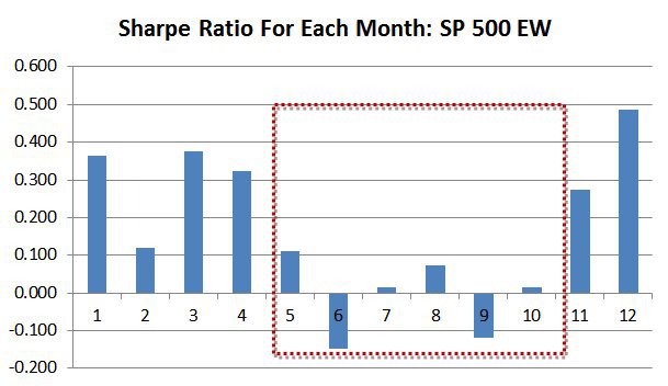
The results are hypothetical results and are NOT an indicator of future results and do NOT represent returns that any investor actually attained. Indexes are unmanaged, do not reflect management or trading fees, and one cannot invest directly in an index. Additional information regarding the construction of these results is available upon request.
This is just data-mining, right?
One very reasonable hypothesis is that the statistics above are a result of data-mining. However, some researchers disagree: For example, Bouman and Jocobsen (2002) attribute this effect to summer vacation, which leads to changing risk aversion and liquidity constraints. They also find that such market anomalies cannot be explained by factors like risk, cross correlation between markets, or the January effect (except US market). Hong and Yu (2009) points out that trading activity is usually lower during summer holiday months. Kamstra, Kramer and Levi (2003) argues that it’s due to mood changes of investors caused by Seasonal Affective Disorder. The debate will rage on.
Reference:
- Bouman and Jocobsen, 2002, The Halloween Indicator, “Sell in May and Go Away”: Another Puzzle”. American Economic Review 92 (5): 1618.
- Jocobsen and Zhang, 2012, The Halloween indicator: Everywhere and All the Time, working paper series.
What will you be doing this May?
About the Author: Wesley Gray, PhD
—
Important Disclosures
For informational and educational purposes only and should not be construed as specific investment, accounting, legal, or tax advice. Certain information is deemed to be reliable, but its accuracy and completeness cannot be guaranteed. Third party information may become outdated or otherwise superseded without notice. Neither the Securities and Exchange Commission (SEC) nor any other federal or state agency has approved, determined the accuracy, or confirmed the adequacy of this article.
The views and opinions expressed herein are those of the author and do not necessarily reflect the views of Alpha Architect, its affiliates or its employees. Our full disclosures are available here. Definitions of common statistics used in our analysis are available here (towards the bottom).
Join thousands of other readers and subscribe to our blog.