Factor Regressions are one way to ascertain a fund’s exposure to certain factors that an investor/advisor may want to allocate towards, such as Value, Momentum, Quality, etc. Luckily, there are some great free tools available online, such as portfoliovisualizer.com, that allows investors to run the regressions for most mutual funds and ETFs. For those interested in diving into the weeds of regressions, we have a post here that has a (1) video explaining how factor regressions work and (2) an excel file to facilitate learning.
However, factor regressions are not perfect.
As I highlighted in a previous post here, titled “Factor Investors Beware: Positive SMB May Not Mean You Own Small-Caps”, the interpretation of factor loadings can be difficult.
Below I highlight two additional issues with factor regressions:(1)
- Loadings are dependent on the definition of a factor
- Loadings have memories and may tell us little about the current portfolio
I dig into each point below.
Issue 1: Factor Loadings are Dependent on the Definition of a Factor
Let’s focus on the value factor.
The traditional HML factor tracks the returns to a long/short portfolio of value stocks formed by sorting stocks on Book-to-Market (B/M) and size ratios. Specifically, the portfolios are formed by sorting the universe into 6 “buckets” based on NYSE breakpoints for both Size and B/M. Most use Ken French’s data, found here. A description of the portfolio is below(2):
The portfolios, which are constructed at the end of each June, are the intersections of 2 portfolios formed on size (market equity, ME) and 3 portfolios formed on the ratio of book equity to market equity (BE/ME). The size breakpoint for year t is the median NYSE market equity at the end of June of year t. BE/ME for June of year t is the book equity for the last fiscal year end in t-1 divided by ME for December of t-1. The BE/ME breakpoints are the 30th and 70th NYSE percentiles.
A visual description of the 6 portfolios is given below:
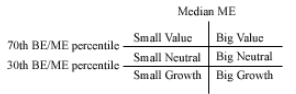
6 portfolios are formed from the universe of all stocks. The HML factor is a long/short portfolio that goes long the (1) Small Value and (2) Big Value portfolios and goes short the (1) Small Growth and (2) Big Growth portfolios shown above. Note that two out of the six portfolios are excluded for the HML factor.
Mathematically, each month the return to the HML portfolio is given by this formula:
HML = 1/2*(Small Value + Big Value) – 1/2*(Small Growth + Big Growth).
When using online tools, such as portfolioviaulizer.com, we get the loading for mutual funds and ETFs on the “value” factor by examining the HML beta loading. As an example, I ran the regression to the Vanguard Value ETF (ticker: VTV) through the analysis tool.
The results are shown below:
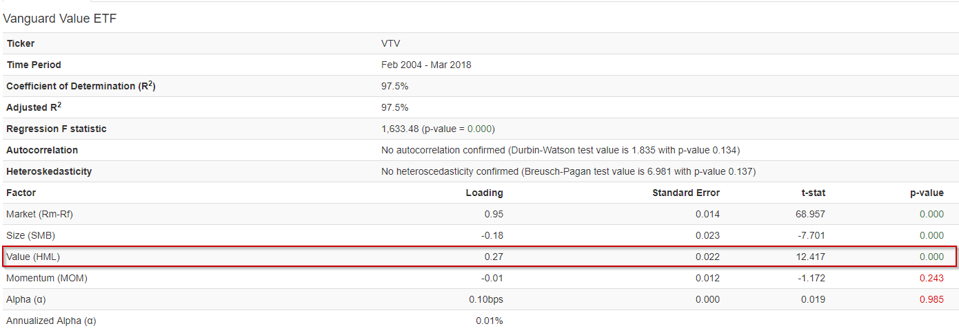
Source: https://www.portfoliovisualizer.com/factor-analysis
As we see above, the VTV ETF has a Value loading of 0.27, with a T-statistic of 12.417! Thus, based on positive and statistically significant loading on the HML factor, one may conclude that this is a value fund worth allocating their investment towards.
However, what if we wanted to invest in a “deep value” portfolio?
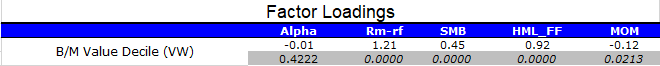
A simple way to do this, while still using publically available data, is to use the top decile of firms ranked on book-to-market from Ken French’s website.(3) Specifically, I regress the value-weight returns to the top decile of firms ranked annually (June 30th) on B/M against the 4-factor model. Below, I show the results of factor regressions from 1/1/1978-12/31/2017, which covers 40 years worth of data. The first row represents the Beta loading on each factor and the second row represents the p-value for significance.
January 1, 1978 to December 31, 2017. The results are hypothetical results and are NOT an indicator of future results and do NOT represent returns that any investor actually attained. Indexes are unmanaged, do not reflect management or trading fees, and one cannot invest directly in an index.
As is shown above, the top decile of B/M firms from Ken French’s site has a Value of HML loading of 0.92, which is highly significant. Not surprisingly, a portfolio formed on B/M has a high loading to the HML L/S return series, which was originally sorted on B/M!
What if B/M based value isn’t your thing?
However, what if you were not a fan of the B/M measure and wanted to use another way to form your value portfolio?
You plan to employ the same methodology–pick the top decile of firms on an alternative value measure. Does that make you any less of a value investor? No! It simply means that you decided to form the value portfolio in an alternative way. For descriptions of value measures, and how they performed in the past, Wes and I have a paper and an update on the various measures. In general, no matter how one measured value in the past, over long time cycles the value paper-portfolios outperformed both (1) growth stocks and (2) the market.
However, how does our factor loading analysis change if we do not use the academic B/M measure to pick the top decile?
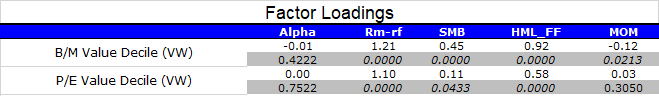
To examine this question, I will use the top decile of firms ranked on earnings-to-price (E/P) from Ken French’s website.(4) This is the inverse of the practitioner favorite P/E multiple. Specifically, I regress the value-weight returns to the top decile of firms ranked annually (June 30th) on E/P against the 4-factor model. Below, I show the results of factor regressions from 1/1/1978-12/31/2017, which covers 40 years worth of data. The first row represents the Beta loading on each factor and the second row represents the p-value for significance.
January 1, 1978 to December 31, 2017. The results are hypothetical results and are NOT an indicator of future results and do NOT represent returns that any investor actually attained. Indexes are unmanaged, do not reflect management or trading fees, and one cannot invest directly in an index.
As shown above, the value decile formed on E/P has a statistically significant value loading of 0.58. Thus, if we were highly focused on the HML Beta loading, it would appear that the top decile of E/P firms has ~ 63% (0.58/0.92) of the exposure to value compared to the top decile on B/M. However, we know that these are both true value portfolios, as both pick the top decile every year on a particular value measure. However, the factor loadings would say otherwise.
To drive home this point, here is the annual performance, gross of any fees or transaction costs, over the 1/1/1978-12/31/2017 time period:
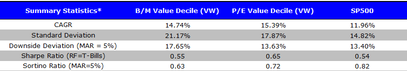
Source: January 1, 1978 to December 31, 2017. The results are hypothetical results and are NOT an indicator of future results and do NOT represent returns that any investor actually attained. Indexes are unmanaged, do not reflect management or trading fees, and one cannot invest directly in an index.
Both value portfolios outperformed the index.(5)
Thus, we have Issue 1: Factor Loadings are Dependent on the Definition of a Factor.
How can we fix this? One way, which is not simple, is to change the definition of the long/short portfolio that we regress the value portfolio against. This would be equivalent to creating a new HML factor formed on another valuation measure, such as E/P or EBIT/TEV. For many, this is not possible.
So how can we ascertain what a fund is doing, and compare it to the “academic” portfolios?
One way to do this is to use our visual active share tool.(6) The tool allows users to plot the “academic” portfolios–to do this, simply start typing “academic” into the ETF/Portfolio search. Each “circle” below represents an individual stock one would be invest, based on the portfolio selected.
Below, I show the three portfolios:
- PB_TOP: Top Decile of Firms sorted on Price to Book (P/B), the invest of B/M.
- PE_TOP: Top Decile of Firms sorted on P/E, the inverse of E/P.
- IWB: iShares Russell 1000 Index ETF
In addition, I have set the x-axis to percentile rank firms on B/M, and the y-axis to percentile rank firms on E/P.

Source: https://tools.alphaarchitect.com/ Accessed on 5/24/18
As we see above, both the “value” paper-portfolios invest in the top decile of firms based on either B/M or P/E multiples. We also notice that (1) there is little overlap relative to the Russell 1000 and (2) using B/M and P/E give different portfolios.
One can now directly examine the “overlap” of the portfolios as well by clicking on the “overlap” tab. As shown below, the exact overlap between the value portfolios is ~43%.
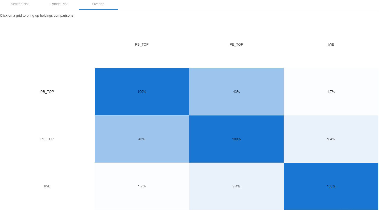
Source: https://tools.alphaarchitect.com/ Accessed on 5/24/18
So while the definition of value may have an effect on the regression results, our tool is one way to assess how much “value” is in a portfolio. The same issue would apply to other factors, and the tool can help by allowing the users to change the x-axis and y-axis to the portfolio characteristics that they would prefer to sort on, as well as comparing against the academic portfolios.
Issue 2: Factor Loadings have Memories
In addition to the definition of a factor being important (issue 1 above), factor loadings will always have a memory. This means that information from 40 years ago will still be embedded in the static factor loading shown if we ran the analysis today. To make this clear, I created a portfolio that every month shifts more and more to the market-cap weighted index–this is a so-called “closet-index” portfolio.
How do I do this?
In month 1 (January 1978), the portfolio is 100% allocated to the B/M Value Decile (VW) as described above. Every month, starting in month 2 (February 1978), an additional 1/480th of the portfolio is allocated to the S&P 500 Total Return Index, which is taken away from the B/M Value Decile portfolio. Thus, the returns in month 2 are (1/480)*(SP500) + (479/480)*(B/M Value Decile). The returns in month 3 (March 1978) are (2/480)*(SP500) + (478/480)*(B/M Value Decile). In the last month (month 480–December 2017), the returns are (479/480)*(SP500) + (1/480)*(B/M Value Decile). So in the next month (1/1/2018), the portfolio is 100% the S&P 500 (note the returns stop on 12/31/2017).
I used the same forty-year time period as above to make the analysis the same–1/1/1978 through 12/31/2017.
To (potentially) make this clearer, I plot the allocation to either the (1) Value portfolio or (2) the S&P500 over time. This is shown below:
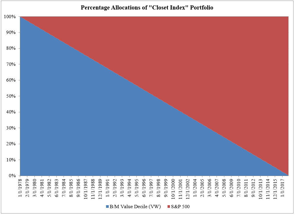
The image above shows how the portfolio linearly transitions from a pure value strategy to the S&P500.
But what would a factor regression tell us about this portfolio? I show the results to the “closet-index” value portfolio described above.
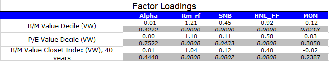
January 1, 1978 to December 31, 2017. The results are hypothetical results and are NOT an indicator of future results and do NOT represent returns that any investor actually attained. Indexes are unmanaged, do not reflect management or trading fees, and one cannot invest directly in an index.
As is shown in the table above, the closet-index value portfolio has a highly significant value (HML) beta loading of 0.40. Thus, in the past, this was a value fund. However, we also know that mechanically this fund has transitioned into the index! Thus, the static HML loading of 0.40 tells us literally nothing about the value portfolio we planned on investing in, based on its 0.40 value loading!
Thus, we have issue 2: Factor loadings have memories and tell us little about the current portfolio
So how can we deal with this issue?
There are two main ways one can deal with this issue.
First, one can examine the Beta loading through “rolling regressions”. What this does is examines the Beta loading throughout time, in an attempt to see if the portfolio changed its allocations (as measured by Betas) over time. Luckily, portfoliovisualizer.com already has this functionality available–all you need to do it click on the “rolling regressions” tab after running a regression. To highlight this, I re-ran the Vanguard Value ETF (VTV) and show the rolling regression Betas below, from portfoliovisualizer.com
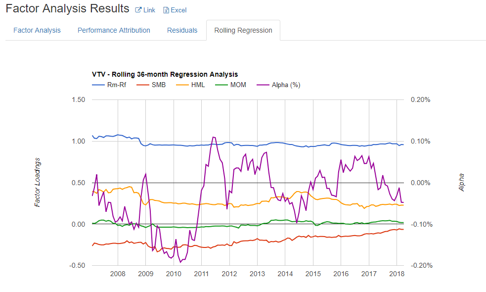
Source: https://www.portfoliovisualizer.com/factor-analysis
As we see above, the Market Beta loadings were fairly stable over time, right around 1.00. The HML (Value) loading was its highest when the fund was initially launched, and while it has declined, but has not deviated greatly.
So let’s examine the rolling regressions on the four paper portfolios we examined above: (1) Top Decile on B/M, (2) Top Decile on E/P, (3) Closet-Index Value, and (4) S&P500. I show the results below. Note that I use a 60-month (5-years) rolling regression, as opposed to 36 months–this is done in an attempt to get more stable beta estimates. Also, I am only plotting the HML loading, since I am plotting these for four different return series.
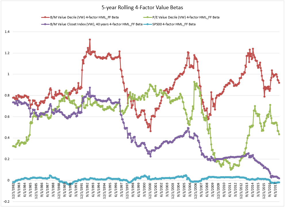
January 1, 1978 to December 31, 2017. The results are hypothetical results and are NOT an indicator of future results and do NOT represent returns that any investor actually attained. Indexes are unmanaged, do not reflect management or trading fees, and one cannot invest directly in an index.
The 5-year rolling-regression 4-factor HML Betas above show us a few things:
- First, the S&P500 (blue line) is very stable and has little or even negative value exposure over time.
- Second, we notice the wild swings for both the red line (which represents the top decile of value firms formed on B/M) and the green line (which represents the top decile of value firms formed on E/P).
- Third, we notice that while the B/M and E/P betas are at times similar, there can be instances where they have massively different HML Betas, such as since the 2008 financial crisis.
Last, and important for addressing issue number 2, when examining the closet-index betas (purple line), we notice a slow downward move towards a lower HML loading–however it is still not zero. This makes sense, as the fund is becoming more and more like the index every month!
Thus, one can use rolling regressions to ascertain whether or not a fund has drastically changed their loadings over time.
However, this still tells us nothing about what the fund is actually invested in today–in my hypothetical closet-index example, on 1/1/18, the fund is 100% the S&P500! Thus, even though we know that (1) the fund has a highly significant 0.40 HML loading and (2) it appears to be reducing its value exposure over time, we have no indication that the fund is simply the S&P500.
So how can we fix this?
A few ways would be to (1) examine the current Active Share of the fund, (2) Dig into the weeds on the holdings relative to the index, or (3) use our visual active share tool.
Below I show the holdings for (1) VTV (Vanguard Value) ETF, (2) SPY (SPDR S&P500) ETF, and (3) PB_TOP (Top Decile of Firms sorted on Price to Book (P/B), the invest of B/M)
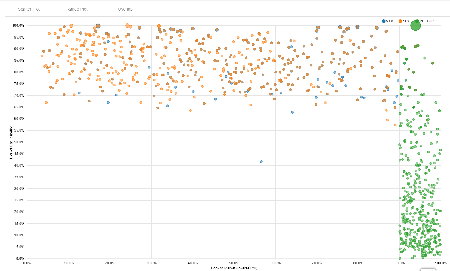
Source: https://tools.alphaarchitect.com/ Accessed on 5/24/18
As we see, there is a pretty high overlap between VTV and SPY, while both are different than the academic top decile on P/B (inverse of B/M). The goal isn’t to pick on Vanguard, as they have a lower fee (0.05%) for the VTV ETF than SPY (0.0945%), rather the goal is to highlight that our tool allows the user to see what the fund is currently holding, and then compare it to a certain benchmark
Conclusion:
Factor regressions are not a panacea. Above, I highlight two issues with factor regressions:
- Loadings are dependent on the definition of a factor
- Loadings have memories and tell us little about the current portfolio
Our visual active share tool allows users to attempt to solve these issues and view the portfolio characteristics. For a deep dive into portfolio characteristics versus factors, see my article here.
About the Author: Jack Vogel, PhD
—
Important Disclosures
For informational and educational purposes only and should not be construed as specific investment, accounting, legal, or tax advice. Certain information is deemed to be reliable, but its accuracy and completeness cannot be guaranteed. Third party information may become outdated or otherwise superseded without notice. Neither the Securities and Exchange Commission (SEC) nor any other federal or state agency has approved, determined the accuracy, or confirmed the adequacy of this article.
The views and opinions expressed herein are those of the author and do not necessarily reflect the views of Alpha Architect, its affiliates or its employees. Our full disclosures are available here. Definitions of common statistics used in our analysis are available here (towards the bottom).
Join thousands of other readers and subscribe to our blog.