Recently, Wes pointed me to this interesting paper by David Rapach, Jack Strauss, Jun Tu and Guofu Zhou: “Dynamic Return Dependencies Across Industries: A Machine Learning Approach.” The paper presents a strategy that forecasts industry returns and shows excellent historical returns. In this piece, we explore the strategy and then try to improve the results with more sophisticated machine learning approaches.
Along the way, we improve upon our previous machine learning primer, and add a few more learning points:
- How to apply machine learning to a practical portfolio problem
- Highlight sample code that can potentially solve financial problems with machine learning techniques
- Gain insights into the benefits and drawbacks of machine learning approaches and their application in financial markets
The summary is as follows (at least for our context):
- Simple linear models are tough to beat and easy to interpret, but plain vanilla machine learning techniques seem to help and are still relatively easy to interpret.
- More sophisticated machine learning models (that include non-linearities) seem to provide better prediction (e.g., lower MSE), but their ability to generate higher Sharpe ratios is questionable.
- Complex machine learning models require a lot of data and a lot of samples. In other words, good for high-frequency-trading, maybe not great for asset allocation or long-term investing.
In Part 1, we’ll discuss the paper. For part Part 2, we talk about backtesting methodology. Parts 3 and 4 are a tutorial on predicting and backtesting using the python sklearn (scikit-learn) and Keras machine learning frameworks. Finally, we’ll conclude with parting advice about pluses and minuses of the machine learning approach.
Everything should be made as simple as possible, but not simpler. — Attributed to Albert Einstein(1)
Part 1: Reviewing “Dynamic Return Dependencies Across Industries: A Machine Learning Approach”
The Rapach, Strauss, Tu, and Zhou paper’s title sounds complicated, but it’s a straightforward industry rotation methodology:
- Use industry returns from Ken French.
- For each month, forecast industry returns using the previous month’s returns from all 30 industries.
- Use lasso regression(2) to select the best subset of predictors for each industry over the history to date, to determine that e.g. Beer is predicted by Food, Clothing, Coal.
A replication(code available here) generates a long/short strategy that returned ~3.5% a year from 1970 to 2016 with ~5.2% annualized volatility, for a Sharpe ratio of 0.67. My numbers — the paper’s numbers in
Table 3 show a higher return (7.3%), similar Sharpe (0.65).
There are 3 reasons I can think of for the difference:
- The authors used R glmnet lasso with AICc, I used python sklearn LassoLarsIC with criterion “aic”. AICc would produce different results from AIC, in addition to the possibility of other implementation differences.
- The authors standardized the predictors. When you do lasso regularization, shrinkage is partly determined by the size of the coefficient. So, if one predictor is 10x another predictor, and its coefficient is 1/10 the size, it will not be subject to the same shrinkage. For this reason, standardizing before the prediction is generally the best practice. However, all our predictors are identical units, and I find that not standardizing yields consistently better results. Standardizing would tend to increase the coefficients on more volatile predictors and subject them to more shrinkage. It’s not obvious that’s theoretically desirable and the machine learning philosophy is to use what works best out-of-sample.
- I wasn’t able to duplicate the author’s return calculations even on raw data where we matched on volatility so there appears to be some slight difference in return methodology.
Source: Druce Vertes, StreetEYE.com. The results are hypothetical results and are NOT an indicator of future results and do NOT represent returns that any investor actually attained. Indexes are unmanaged, do not reflect management or trading fees, and one cannot invest directly in an index.
The S&P yielded a little over 7% excess return over that period with a little under 17% volatility for a Sharpe ratio of 0.42 (from Aswath Damodaran’s data). A Sharpe of 0.8 over the long term would be Buffett-like. But our strategy is a theoretical zero-investment portfolio. Pick 6 industries at random to go long and 6 at random to go short, you should expect a return of 0. Lever up our strategy’s return to match S&P volatility, and you would have earned an excess return of ~11.4%. As Larry David would say, “That’s pretty pretty good.”
Even after margin, slippage, this result suggests that historically there were patterns in industry rotation that could have been exploited.
Interestingly, this portfolio performance occurs despite very low R2 in industry return prediction: the highest R2s are around 8% (The paper’s Table 2) and the mean is around 4%. One interpretation is that maybe you can be significantly more accurate than chance in predicting the winner of a season’s football games while being only slightly more accurate than chance in predicting each game’s score. It is possible for your rankings to be accurate, even if your predictions of the performance scores are not. Even so, explaining 4% of variation in-sample doesn’t seem like the edge to turn a dart-thrower into a Warren Buffett. My intuition fails a little here.
Another interesting aspect of the paper is that it demonstrates the effectiveness of the lasso predictor selection. Per the paper’s Table 3, and the chart below, lasso works significantly better than just regressing monthly returns against all industries.

Source: Druce Vertes, StreetEYE.com. The results are hypothetical results and are NOT an indicator of future results and do NOT represent returns that any investor actually attained. Indexes are unmanaged, do not reflect management or trading fees, and one cannot invest directly in an index.
There is a good reason for this result: When you fit against all 30 predictors — versus a subset of the best predictors — you will get a higher in-sample R2. But then the model will not predict as well out-of-sample. You add less informative predictors, your model will overfit them in-sample and not work as well out-of-sample. Lasso effectiveness is shown in the chart above comparing lasso subset selection followed by OLS prediction, versus pure lasso, and then pure OLS.
It’s an interesting analysis and interesting result. But the machine learning in the title is limited to lasso predictor selection. Let’s break this down “Barney Style”(3) and learn how to estimate time-series forecasts with machine learning using Scikit-learn (Python sklearn module) and Keras machine learning estimators.
Part 2 – Backtesting and cross-validation.
Let’s look at a typical machine learning cross-validation workflow. This will illustrate the key concepts before moving on to portfolio backtesting, which is more complicated.
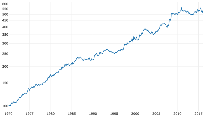
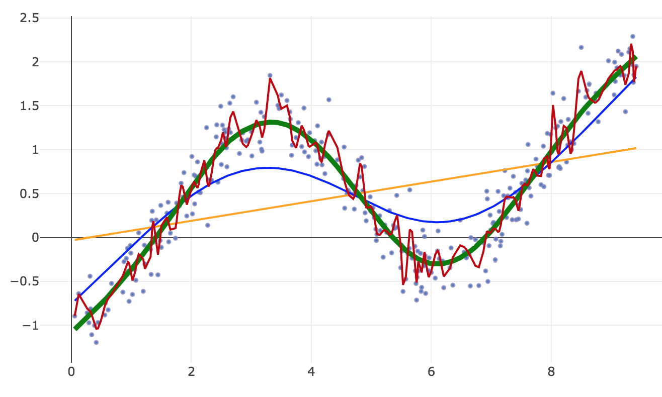
We generate some data that follows a sine wave, plus a trend, plus random noise.
The results are hypothetical results and are NOT an indicator of future results and do NOT represent returns that any investor actually attained. Indexes are unmanaged, do not reflect management or trading fees, and one cannot invest directly in an index.
If we do linear regression, we get the orange straight line (the trend).
If we go non-linear and fit all the data with many degrees of freedom, we get the curviest, noisy red line, which overfits the data.
With machine learning algorithms, there is generally a way to tune the degree of nonlinearity. How do we choose the best fit? Using cross-validation.
In the simplest form of cross-validation, we take out 20% of our data at random to use for cross-validation. We also take out 20% at random for test. We fit on the remaining 60%.
- We start with linear regression and measure the error in the cross-validation set.
- We repeatedly increase the degree of nonlinearity and check fit in the cross-validation set.
- We stop when we get the best fit in cross-validation, i.e when a measure of forecast error like MSE reaches a minimum — the thick green line.
- Finally, we predict on our test set and measure our test accuracy, which should be close to our cross-validation score. This is our best estimate of our model’s performance on out-of-sample data.
We never looked at our test data before, so effectively it is out-of-sample data.(4) A few rules:
- We never make a decision about our model based on in-sample training metrics.
- We only use cross-validation performance to optimize parameters and select a model.
- We never make a decision about our model based on test data.
- We set test data aside until our model is finalized.
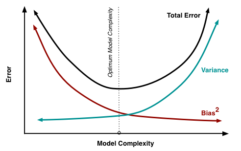
If we do it right, our model should be close to the optimum point in the bias-variance curve (via Scott Fortmann-Roe). This illustrates how, as you increase your model’s complexity (degree of nonlinearity, number of knots/kinks, number of parameters), your accuracy initially increases. Your model is less biased to an unrealistically simple model assumption. But as you continue to increase complexity, variance increases. You have a lot of model parameters and not a lot of data, the model tends to overfit variations in the data, the error bars around your estimates grow larger, and if you resampled you’d get different estimates.
 I hope this convinces you that using a nonlinear model with careful cross-validation can control overfitting and may improve forecasts.
Complex nonlinear models don’t necessarily overfit, and simple linear models don’t guarantee against overfitting. When scientists use small samples, test many hypotheses, and publish only the ones with statistically significant p-values, they get the pizza papers and power poses. (These practices have been widespread, and these unfortunate researchers were made examples of, not because they were among the worst scientists, but because they were among the most popular.) If you p-hack in-sample p-values, and don’t validate outside your training data, even linear models will be overfitted to training data because you only publish models that show the luckiest match to the training data.
But if you are careful, you can use nonlinear models and machine learning to improve prediction without overfitting. If the underlying reality is nonlinear, a nonlinear model will be closer to reality and the predictions will perform better out-of-sample.
Now let’s talk about backtesting time series forecasts using walk-forward cross-validation.
Simple cross-validation would be to set aside 20% of the data at random. However, with time series data, you have to consider serial correlation. We often want to fit models that use prior period data. If we pick 20% of the rows at random for cross-validation, those rows leak information that is also in the cross-validation and test sets.
To minimize snooping, we use walk-forward cross-validation:
- Divide the data into 4 folds, without randomizing or re-ordering.
- Train the model on fold 1, use the resulting model to generate an evaluation score on the data in fold 2. (e.g. MSE or R2)
- Train the model on folds 1 and 2, use the resulting model to generate an evaluation score on fold 3.
- Train the model on folds 1, 2, and 3, use the resulting model to generate an evaluation score on fold 4.
- Average the 3 scores.
We can then optimize our model by iteratively evaluating different model specifications, and selecting the model that has the best performance in cross-validation.
Finally, we run a backtest simulation on the best model. We train from January 1960 to December 1969. We use the resulting model to predict January 1970. Using that prediction, we pick the top 6 industries to go long and the bottom 6 industries to go short. Then we train from January 1960 to January 1970, and use that model to predict and pick the portfolio for February 1970, and so on.(5)
Part 3 – Prediction using sklearn.
So, now let’s implement our methodology using Python sklearn machine learning algorithms (viewable notebook and Git repository).
The first thing I often do in attacking a machine learning problem is to enumerate all the applicable sklearn algorithms, run them all, and see which ones perform well, and get a feel for how well off-the-shelf algorithms perform with default settings (hyperparameters). If one seems promising, we tune hyperparameters using cross-validation.
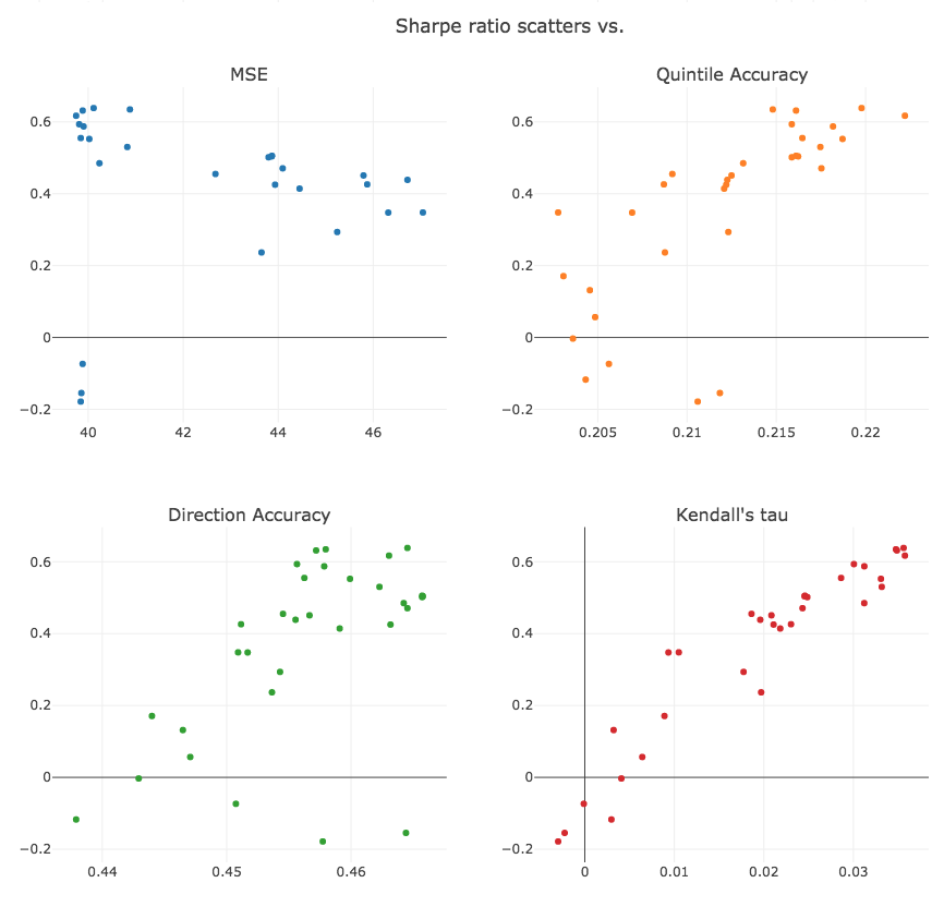
One thing that jumps out is that the relationship between MSE and Sharpe is highly imperfect.
Recall that we go short the bottom quintile and long the top quintile. When we reduce MSE error, it only improves performance if 1) some predictions get correctly moved into the top or bottom quintile and 2) incorrect predictions get moved out. It’s possible to reduce MSE error without improving performance. Of course, if MSE is reduced to 0, we will correctly predict all rankings. But we are far from 0 MSE.
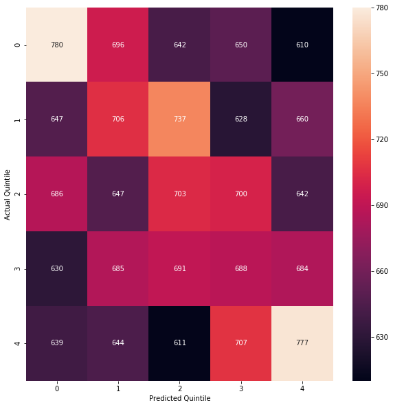
To get a better picture of how the predictions impact returns, we can generate a confusion matrix which shows how the predicted quintiles line up with the observed actual quintiles.
For our lasso/OLS model:
The results are hypothetical results and are NOT an indicator of future results and do NOT represent returns that any investor actually attained. Indexes are unmanaged, do not reflect management or trading fees, and one cannot invest directly in an index.
If our quintile predictions were random, we would expect 4% to fall in a given quintile square, or about 675 predictions. The correct predictions on the diagonal are significantly better. Using a chi-square test, the null hypothesis that a random quintile distribution would classify the 1st quintile as shown, with 780 true positives, is rejected, with a p-value of about 0.000017.
We can also calculate accuracy in classifying into long/short/flat, by e.g. comparing the predicted top 6 with the actual top 6. The true shorts are the correctly classified bottom quintile at top left, true longs are the correctly classified top quintile bottom right, and true flats are the 3×3 square in the middle. If we classified randomly we should get 0.2*0.2 + 0.6*0.6 + 0.2*0.2 = 44% correct, but we got 45.8%.
Finally, we observe that we are really using our regression as a proxy to classify or rank the industries. Kendall’s tau is a metric used to evaluate ranking accuracy. It tells us, if we pick two industries at random, then given their correct ranking, what is the expected value of the predicted relative ranking? If the predicted ranking is always correct, Kendall’s tau is 1.0. If the predicted ranking is always the reverse of the observed ranking, Kendall’s tau is -1.0. If the predicted ranking gives no information, Kendall’s tau is 0. It can be interpreted similarly to correlation, but for ranking. We compute Kendall’s tau between the correct ranking and the predicted ranking, to give us a measure of ranking accuracy over the full 30 buckets.
If we run a scatter, we observe that the average Kendall’s tau over all rows corresponds quite well with the Sharpe ratio, better than the accuracy measures, which are in turn better than MSE.
Correlation matrix:
| sharpe | mse | kendalltau | quantile_score | direction_score | truepositive_score | |
|---|---|---|---|---|---|---|
| sharpe | 1.000 | -0.348 | 0.947 | 0.727 | 0.560 | 0.838 |
| mse | -0.348 | 1.000 | -0.251 | -0.258 | -0.459 | -0.425 |
| kendalltau | 0.947 | -0.251 | 1.000 | 0.816 | 0.589 | 0.865 |
| quantile_score | 0.727 | -0.258 | 0.816 | 1.000 | 0.821 | 0.903 |
| direction_score | 0.560 | -0.459 | 0.589 | 0.821 | 1.000 | 0.905 |
| truepositive_score | 0.838 | -0.425 | 0.865 | 0.903 | 0.905 | 1.000 |
We also notice in our table of sklearn results that ElasticNet does pretty well(6). ElasticNet is a generalization of lasso to include a combination of L1 (lasso) and L2 (ridge) regularization.(7)
Let’s try ElasticNet instead of lasso/OLS. We have 2 parameters, alpha, the size of the regularization penalty; and l1_ratio, the size of L1 relative to L2. If l1_ratio=1, we are doing lasso L1 regularization, if l1_ratio=0 we are doing L2 ridge regression. If l1_ratio is between those extremes it combines both L1 and L2 regularization. We vary these parameters and on our best parameter combination, we see an improvement to almost 0.7 Sharpe.
| alpha | l1_ratio | mse | sharpe | quantile_score | direction_score | kendalltau | truepositive_score | |
|---|---|---|---|---|---|---|---|---|
| 22 | 10 | 0.100 | 39.725 | 0.695 | 0.221 | 0.465 | 0.042 | 250.800 |
| 30 | 30 | 0.010 | 39.660 | 0.650 | 0.224 | 0.468 | 0.042 | 258.800 |
| 9 | 1 | 1.000 | 40.114 | 0.639 | 0.220 | 0.465 | 0.036 | 237.800 |
| 8 | 1 | 0.990 | 40.123 | 0.621 | 0.220 | 0.465 | 0.035 | 236.800 |
| 13 | 3 | 0.500 | 39.762 | 0.617 | 0.223 | 0.464 | 0.037 | 236.800 |
Here is a visualization of the result:

The results are hypothetical results and are NOT an indicator of future results and do NOT represent returns that any investor actually attained. Indexes are unmanaged, do not reflect management or trading fees, and one cannot invest directly in an index. Additional information regarding the construction of these results is available upon request.
So using 1) L1 + L2 regularization and 2) cross-validation to optimize L1 and L2 penalties, we got a slightly better result than lasso subset selection and OLS.
ElasticNet is still an additive linear model. It doesn’t model nonlinear relationships or interactions. We could try to tune other nonlinear models. We could also take our 30 predictors, add higher-order terms and interactions between all of them, and run ElasticNet. We’ll leave this as an exercise. (We tried to tune MLPRegressor, and we tried adding squares and pair interactions to ElasticNet, but neither seemed to work very well).
Part 4 – Prediction using Keras.
The Keras machine learning framework provides flexibility to architect custom neural networks, loss functions, optimizers, and also runs on GPU so it trains complex networks much faster than sklearn.(8)
On the other hand, it takes longer to initialize each model. In the sklearn backtest, we run 30 regression models at each timestep, one for industry response variable. We can take advantage of Keras’s flexibility to share the lowest layers between predictions and run 30 predictions simultaneously.
Neural network model:
- Input 30 predictors
- 1 or more fully connected dense relu (rectified linear) layers
- 30 linear output layers on the last relu layer to predict the output of regression
- Minimize MSE loss (average MSE across all 30 outputs simultaneously)
We test a number of neural network architectures to find one with the best bias/variance tradeoff:
- 1, 2, 3 layers.
- 1, 2, 4, 8, 16 units per layer.
- L1_L2 Regularization similar to ElasticNet, with penalties of 0.0, 0.1, 0.3, 1, 3, 10, 30, 100. There is no l1_ratio parameter, we cannot independently set L1 and L2 penalties, penalties are equal when the coefficient is 1.
We try all combinations of these hyperparameters in a big loop; we run walk-forward cross-validation using each combination; we put them in a table and sort by cross-validation MSE:
| layers | layer_size | reg_penalty | mse | sharpe | quantile_score | direction_score | kendalltau | truepositive_score | |
|---|---|---|---|---|---|---|---|---|---|
| 7 | 1 | 1 | 100.000 | 39.550 | -0.043 | 0.204 | 0.450 | 0.002 | 54.200 |
| 31 | 1 | 8 | 100.000 | 39.551 | 0.267 | 0.215 | 0.460 | 0.009 | 142.200 |
| 23 | 1 | 4 | 100.000 | 39.553 | -0.133 | 0.204 | 0.451 | -0.004 | 39.200 |
| 103 | 3 | 4 | 100.000 | 39.553 | -0.079 | 0.206 | 0.454 | -0.001 | 71.200 |
| 5 | 1 | 1 | 10.000 | 39.556 | -0.076 | 0.206 | 0.451 | 0.000 | 61.200 |
| 15 | 1 | 2 | 100.000 | 39.559 | -0.104 | 0.204 | 0.451 | -0.003 | 47.200 |
| 95 | 3 | 2 | 100.000 | 39.559 | -0.061 | 0.208 | 0.455 | -0.001 | 84.200 |
| 46 | 2 | 1 | 30.000 | 39.560 | -0.087 | 0.209 | 0.457 | -0.001 | 92.200 |
and by Sharpe
| layers | layer_size | reg_penalty | mse | sharpe | quantile_score | direction_score | kendalltau | truepositive_score | |
|---|---|---|---|---|---|---|---|---|---|
| 74 | 2 | 16 | 0.300 | 116.058 | 0.779 | 0.222 | 0.469 | 0.039 | 274.200 |
| 75 | 2 | 16 | 1.000 | 84.126 | 0.491 | 0.219 | 0.465 | 0.027 | 212.200 |
| 28 | 1 | 8 | 3.000 | 53.849 | 0.472 | 0.217 | 0.459 | 0.020 | 155.200 |
| 24 | 1 | 8 | 0.000 | 64.602 | 0.426 | 0.215 | 0.461 | 0.017 | 177.200 |
| 38 | 1 | 16 | 30.000 | 40.933 | 0.411 | 0.213 | 0.454 | 0.023 | 126.200 |
| 108 | 3 | 8 | 3.000 | 78.105 | 0.395 | 0.210 | 0.453 | 0.019 | 124.200 |
| 18 | 1 | 4 | 0.300 | 49.558 | 0.381 | 0.215 | 0.458 | 0.015 | 143.200 |
| 76 | 2 | 16 | 3.000 | 85.776 | 0.374 | 0.211 | 0.456 | 0.019 | 154.200 |
We can also plot the results on a heat map to get a feel for persistent patterns and discard outliers:
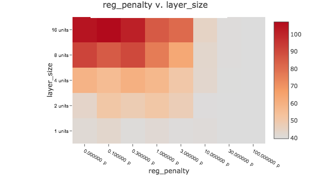
We see a lot of low MSEs clustered around 39.5 for high-bias models (fewer layers, fewer units, higher regularization penalty). We generally don’t see very good Sharpes, and they are not associated with the lowest MSEs. We actually see one very good Sharpe of 0.779 inexplicably associated with a very high MSE of 116. When we run the full backtest using the hyperparameters, instead of the quick-and-dirty walk-forward cross-validation, we get a much lower Sharpe. Given high MSE and poor backtest I think we have to dismiss it as a lucky cross-validation artifact.
We did achieve many lower out-of-sample MSEs than we saw with lasso/OLS and ElasticNet but they yielded poor Sharpe ratios. I interpret this to mean nonlinearity allows the neural net model to minimize MSE better than linear models, which is its objective. However, it seems to achieve low MSE in a way which does not translate to good rankings (Kendall’s tau) or returns (Sharpe). It wins the MSE game but loses the Sharpe meta-game. Perhaps MSE is a poor choice of objective function because it is not strongly associated with our real-world objective (mean return and Sharpe) and it leads a more flexible model astray. Perhaps the nonlinear model adds no value because there is an essentially linear underlying relationship between performance and predictors. Perhaps both. It’s not what I expected.
An alternative would be to minimize an objective more directly linked to performance. We could use a classification model instead of a regression model, sorting into quintile buckets by predicting bucket probability and minimizing cross-entropy, which might be a more appropriate objective function. On the other hand, you lose a lot of information granularity and need more data to train a classifier on quintile buckets instead of return magnitudes. Ordinal regression, which is similar to classification but rank-aware, is another possibility. A final alternative would be to try to maximize returns or Sharpe directly, instead of a proxy like MSE. It would require a custom deep network. It would need a well-designed portfolio function. Top 6 – bottom 6 is inherently not strictly convex everywhere; as you perturb your coefficients slightly, nothing happens to returns until an industry gets bumped to another bucket. (This the reason we typically use a well-behaved objective like MSE as a proxy to optimize what we really care about, like mean return or Sharpe.)
But for this initial blog post, we’ve gone far enough down the rabbit hole and hopefully given you starter code and a feel for how it works.
Part 5 – Conclusion
What did we learn?
- Lasso works. For linear models, regularization improves prediction. ElasticNet performed best, followed by Lasso/OLS, followed by pure lasso, followed by vanilla OLS.
- We showed how to use walk-forward validation to select optimal hyperparameters and backtest using sklearn and Keras.
- We didn’t get performance improvement with our first Keras neural network regression model. Perhaps we need alternative algos and have problematic specifications?
- Did it work well enough to use this model in a portfolio? No. Predicting 30 industries using 1 month of historical returns is a simple model. We’d probably want to see better performance (Sharpe > 1) to provide a higher margin for slippage, costs, probable mean reversion; better recent performance (no fall-off after financial crisis). But for such a simple model, it’s a good result and demonstration of the methodology.
- It’s worth nothing that the most important part of a model is selecting the predictors, which we took as given since we are comparing machine learning algos to an existing linear model. Otherwise, we would do exploratory analysis on possible predictors, look at trends, seasonality, how the predictors relate to each other and the response at different lags, experiment with dimensionality reduction using PCA and neural network autoencoding.
I hope we showed that it’s possible to get better potential predictions with machine learning models.
What are the downsides of machine learning?
- Complexity. It’s much more time-consuming to develop, optimize and test models. Models have a lot of hyperparameter combinations to optimize. Models take a long time to train. Check the times in the notebook, you have to be patient and run a lot of overnight jobs!
- You need a lot of data. The more complex your model, the more data you need.(9) Neural networks tend to need more data than one might reasonably expect. In hindsight, this data set may not be a great example to highlight benefits of neural networks. We might have done better with e.g. weekly or daily data.
- Failure modes are hinky. With linear regression, if you have sufficient independent data, you get a fast closed-form solution. Numerical optimization by stochastic gradient descent is a slower, more approximate process. Your neural network may get a very slightly different, but still pretty good result each time. Sometimes, you might also get a much worse result than you expect – if the objective is not well-behaved (adequately convex everywhere) the optimizer can get stuck at a local minimum or even diverge. When you don’t have plenty of data, neural networks get…hinky.
- Opaque attribution. Increased complexity means you don’t always get simple explanations. With linear models, a constant slope means that if you perturb any x by delta, y always changes by the same amount. When you go nonlinear and add complex interactions between predictors, attribution is not typically human-understandable. You can compute a slope for small changes in underlying parameters, but a small distance away those slopes may be very different. With linear regression, you may get bad predictions but you know why. Your model is simple, and you have error bars (which are accurate modulo all your violations of assumptions of OLS). With machine learning, you may get more accurate predictions but not know why. Pick your poison!
- Brittleness. Nonlinearity means flexibility. It means small changes to inputs can significantly change responses. A higher-variance model is great if it matches the underlying reality. But if it reflects an artifact in training data, or you come across a never-seen out-of-sample regime, your real-world predictions may be poor.
Two common criticisms of machine learning are overfitting and black-box attribution. Von Neumann said the following:
With four parameters I can fit an elephant, and with five I can make him wiggle his trunk.
Meaning, multiple regression becomes unreliable in most settings with more than about 3 predictors.
With today’s improvements in machine learning, and with a lot of good data and careful cross-validation, we can now make reliable forecasts on datasets with many noisy predictors and avoid overfitting. But in a sense, all real-world models are overfitted to the history we have experienced. In economics and finance, for many important questions, we just don’t have historical data encompassing all possible system regimes. We may not have covariance stationarity, as long-term fundamental trends like globalization, fixed vs. floating exchange rates, huge changes in the structure of the global economy etc. change underlying relationships between time series over time.
Like the quote attributed to Bohr says, “It is difficult to make predictions, especially about the future.”(10)
If you have high confidence underlying reality is simple additive causality and linear relationships, you don’t need and don’t want a complex model.(11) On the other hand, if underlying reality is messy with complex nonlinear interactions, the simple model won’t work very well. A nonlinear model will work better, and the lack of simple attribution is just a feature of reality where simple outcomes can have complex causes.
Sometimes reality is an elephant wiggling his trunk, and these days, if you have a lot of data, with machine learning, for the first time, we can model it usefully.
If you have a portfolio strategy where you have a lot of data and make a lot of little decisions, like high-frequency trading, you probably don’t care too much about attribution. You keep your bets small, and if it stops working for longer than can be accounted for by variance, you modify it or stop using it.
But for a long-term strategy, like asset allocation or a Warren Buffett 20-slot punch card, when you try to figure out what baskets to put all your eggs in, by the time you find out it didn’t work, you are broke, or fired. In this type of application it might be interesting to know what machine learning recommends, but you probably want to know the reason for the recommendation, and that it is based on a dynamic that is likely to be persistent, like an exploitable human cognitive bias or market inefficiency, and ultimately make your own reasoned decision.
Bottom line: as Einstein said in the opening quote, make your model as simple as possible, but not simpler. For success, you need both data and theory. If you only follow the data, your model cannot reason about never-seen data regimes. Big data is no substitute for understanding underlying dynamics.
But if you only have a theory and don’t tune the theory to the data as well as possible, you don’t have an evidence-based process.
Machine learning may improve investment predictions and outcomes when underlying reality is nonlinear.
I hope this helps you on your machine learning journey.
Code is here.
Thanks to David Rapach for correcting an earlier version of this post with misunderstandings about the methodology, and thanks to my machine learning study partner Eric Gotthelf of Columbia Astronomy for helpful comments.
References[+]
| ↑1 | Quote Investigator: Maybe Einstein. |
|---|---|
| ↑2 | Lasso is a statistical learning algorithm that uses ‘shrinkage’ to select the most important predictors. Instead of minimizing mean squared error (MSE), we minimize MSE, subject to sum of abs(each coefficient) < t, where t is some regularization parameter.
|
| ↑3 | A Marine Corps term Wes taught me. The idea is to start with the basics. This way even a stupid purple dinosaur could understand what is going on |
| ↑4 | In practice you may have to think carefully about whether the test data is representative of out-of-sample data and not overly correlated with training/cross-validation. You also want to avoid pressing your luck and stop a little before reaching the absolute minimum CV error. Bottom line, test error should be modestly higher than CV error, either because you stopped before the absolute minimum CV error, or you didn’t and probably picked a model that was a little bit luckier in CV than in test. |
| ↑5 | Perceptive readers will note that this backtest is identical to walk-forward cross-validation with 1 observation per fold. We can view the described walk-forward cross-validation methodology as a quick-and-dirty backtest that forecasts many months at a time instead of just one. |
| ↑6 | Others do well too but they are related, i.e. variants of lasso, and ElasticNet is standard, popular, related to the paper’s lasso methodology, and important for our purposes, highly tunable. |
| ↑7 | Lasso will tend to shrink the coefficients that give the least bang for the buck, in terms of MSE improvement per coefficient unit. Ridge regression will tend to shrink large coefficients in favor of smaller ones. It minimizes the sum of squares of the coefficients or their 2-norm or Euclidean distance. In a right triangle, shrinking the shortest side gives the least bang for the buck in shrinking the hypotenuse. By adding both L1 and L2 penalties and choosing the best combination in cross-validation, we are shrinking coefficients that don’t add much value, with an additional bias toward shrinking large coefficients. For more on lasso, ridge regression, regularization, etc., see The Elements of Statistical Learning, by Trevor Hastie, Robert Tibshirani, Jerome Friedman. This is also a good video on L1/L2 regularization. |
| ↑8 | Sklearn is considered ‘off-the-shelf’ machine learning. It doesn’t run on GPU. TensorFlow, which allows you to create arbitrary computations to run very efficiently on large datasets using your GPU, is a low-level machine learning framework. Keras is a high-level machine learning framework that runs on top of TensorFlow. (Historically, on other low-level frameworks, but TensorFlow has become the most widely adopted low-level framework.) Keras makes it very easy to architect complex algorithms, while also exposing the low-level TensorFlow plumbing. Sklearn is incredibly powerful, but sometimes doesn’t let you tune flexibly, for instance, the MLPregressor neural network only has L2 regularization. A snob might view sklearn as training wheels, while state-of-the-art machine learning research would typically be done in Keras and TensorFlow. |
| ↑9 | Running our mad science experiments on sample data, some of the neural networks produce worse results than one might expect. I ended up creating the sine-wave example in R using smoothing splines. I tried neural networks and as I added complexity I expected to trace out the bias/variance curve smoothly, but it was very noisy. As you increase the size of your neural network, sometimes you get a good result, then a bad one, then a much better one. |
| ↑10 | Quote Investigator: Maybe not Niels Bohr. |
| ↑11 | If done carefully, machine learning prediction should not lead you too far astray if you do it right. At worst the simple model falls out of your complex algorithm, or you will find the complex model doesn’t perform better than the simpler model and throw it out. |
About the Author: Druce Vertes
—
Important Disclosures
For informational and educational purposes only and should not be construed as specific investment, accounting, legal, or tax advice. Certain information is deemed to be reliable, but its accuracy and completeness cannot be guaranteed. Third party information may become outdated or otherwise superseded without notice. Neither the Securities and Exchange Commission (SEC) nor any other federal or state agency has approved, determined the accuracy, or confirmed the adequacy of this article.
The views and opinions expressed herein are those of the author and do not necessarily reflect the views of Alpha Architect, its affiliates or its employees. Our full disclosures are available here. Definitions of common statistics used in our analysis are available here (towards the bottom).
Join thousands of other readers and subscribe to our blog.