Using Flexible Spending to Achieve Financial Goals

Financial planning and specifically portfolio “safe” withdrawal rates are often viewed and analyzed from the perspective of rigid rules that can’t be broken – i.e., you will take an inflation adjusted 4% of starting portfolio value every year regardless of past performance. This rigidity is beneficial in understanding how much someone might need to accumulate before they contemplate retirement, but it is a pretty poor reflection of how someone would actually navigate retirement.

Thankfully, there has been some financial planning articles written about how to change withdrawal amounts over time to increase the initial withdrawal rate. The best known of these articles is by Guyton and Klinger (GK) from the March 2006 Journal of Financial Planning which can be found here. GK found that one can increase the initial withdrawal rate from 4% to slightly more than 5% by utilizing their flexible spending rules…cool right?

Well, not so fast.

Spending Flexibility Can Be Harsh

The blog earlyretirementnow has a great blog post (one of a long series on withdrawal rates) that looks at the GK spending rules in-depth. Although written with some disdain, the point of the post is great – GK rules allow a retiree to start with a 5% initial withdrawal rate but there may be some pretty drastic changes to spending along the way.

Here is a paragraph from the conclusion of the blog post:

Talking about skeletons, here’s more data from the GK horror show: The decline of withdrawals from peak to bottom is a staggering 59%, 66%, and 69%, respectively. Ouch! If you thought that the $1,000,000 portfolio can afford you a $50,000 per year lifestyle using GK, you better plan for a few sub-$20k years and an entire decade (!) of sub-$25k p.a. withdrawals. Suddenly the Guyton-Klinger method doesn’t look so hot anymore.

It should be clear from earlyretirementnow’s post that GK is a great starting point for flexible spending but it is not a panacea as most people wouldn’t want the dramatic spending cuts that could be required! So where does that leave us as investors or financial planning practioners?

I decided to use some idle curiosity and personal experience and attempt to model a more realistic set of flexible spending rules to see how results changed.

Modeling a More Realistic Flexible Spending Program

First, let’s start with some assumptions and a baseline scenario (inflexible scenario) to compare the results against. I have assumed that a retiree with 30 year retirement horizon owns an initial $1,000,000 investment portfolio with an expected real return of 4% and a standard deviation of 10%. This retiree will make a $40,000 per year real withdrawal (i.e., a classic 4% initial withdrawal rate) every year. This withdrawal is comprised of $32,000 of living expenses, $4,000 of auto lease payments and $4,000 of vacation expenses.

Next, we consider areas where a retiree would have some spending flexibility (all other assumptions are maintained). In order to provide some benefit from flexibility, the spending must have two qualities 1) the expense must be a material amount of the budget and 2) must have have some acceptable substitute.

In my experience, there are two expenditures most retirees incur that satisfy both criteria 1) vacations and 2) auto purchases. Both of these expenses have substitutes (you can do a Disney vacations at different price levels or even substitute a Six Flags trip for Disney. You can also buy a Toyota instead of a Lexus or a used car instead of a new car) and both expense types are normally material parts of a budget (most budgeting advice/actual budgets have each expenditure equal to about 10% of gross income each year).

Now let’s create some flexible spending rules for those two categories (shown in the table below):

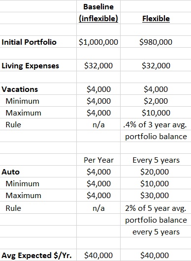
Our flexible investor will plan on buying a car every 5 years (starting at time 0) for a real $20,000 (this makes their initial portfolio $980,000 instead of $1,000,000). In this way, the total car expenditures would be the same as our baseline example, however, the flexible investor will spend 2% of the trailing 5 year average real portfolio balance. If the amount from the rule is less than a real $10,000 then the investor will still spend a real $10,000 on the car. Additionally, if the 2% of trailing 5 year average is more than a real $30,000 then the investor will only spend a real $30,000 on the car. In this way, the investor will always have a car to use but this portion of their withdrawal is variable based on actual portfolio performance.

Additionally, we will assume that our flexible investor will plan on spending the same $4,000 per year on vacations, but they will let their vacation budget vary and be equal to 0.4% of the average 3 year trailing real portfolio value. If the formula amount is less than a real $2,000 then spend a real $2,000 and if if the formula leads to an amount over a real $10,000 then spend only a real $10,000.

So to recap our flexible spending rules – Our flexible investor has made 20% of the annual budget ($4,000/year for autos ($20,000 every 5 years) and $4,000/year for vacations) dependent on their portfolio performance using two different spending rules each with a minimum floor and a maximum cap.

Now let’s take a look at the results:

We can look at the results two different ways 1) see how the flexible spending rules changes the success rate or 2) how much more can an investor spend on Living Expenses (total expenses less vacations and car purchase) when they have a flexible rule for vacations and car purchases (20% of their expenditures)?

First, we see that our baseline (inflexible 4% withdrawal rate) has a success rate of 83.6% of the simulations. This success rate is less than what is cited for most of the 4% initial withdrawal rate articles because I am assuming a real 4% rate of return instead of the historical average of 5% real. For this 83.6% success rate, the investor is able to always withdrawal $40,000 from their portfolio every year ($4,000 for vacations, $4,000 for car lease and $32,000 for living expenses).

Next, we look at the results for changing the modeled success rate – If the flexible investor is OK not maximizing their spending during their retirement then they are able to have a 92.8% success rate! On average, we see that they are able to spend almost as much as our baseline scenario with $39,853 per year in spending ($3,912 for vacations, $3,942 for car purchase and $32,000 for living expenses) vs. $40,000 in total spending for our baseline scenario. However, there are some years where they spend as little as $36,000 ($2,000 for vacations, $2,000 for car purchases and $32,000 for living expenses). This increase in success rates doesn’t come without a cost!

So how much can a flexible investor spend and keep the same success rate the same as our baseline (I think this is a more important question)? The results show that the flexible investor was able to increase the Living Expenses to $37,000 per year! This means that on average, the flexible investor was able to spend a total of $44,853 from the portfolio ($37,000 of Living Expenses, $3,912 for vacations and $3,942 for car purchase) for a 4.49% withdrawal rate! Additionally, even assuming the minimum amount for vacations ($2,000) and car purchase ($10,000 every 5 years or $2,000 per year) the flexible investor can spend $41,000 per year which is still IN EXCESS of the baseline scenario!

In summary, for an investor or retiree who is willing to embrace flexible spending policies based on portfolio performance for certain expenditures (material amount of money and have good substitutes), they can either improve their success rate or materially increase their initial withdrawal rate from their portfolio. Flexibility is powerful!