- Henry R. Oppenheimer
- A version of this paper can be found here
- Want to read our summaries of academic finance papers? Check out our Academic Research Insight category
Introduction
“Ben Graham’s Net Current Asset Values: A Performance Update” by Henry R. Oppenheimer was published in the Financial Analysts Journal, Vol. 42, No. 6 (Nov. – Dec. 1986). The study examined the performance of securities that were trading at no more than two-thirds of their “net current asset value (NAV)” during the 13 year period from 1970-82 period in the US.
Our objective was to analyze the study itself; determine its reliability, draw our own conclusions and glean, if any, actionable advice for the practitioner of the “net net” method of investing.
Please note, the terms “NAV” and “net nets” are used interchangeably throughout the analysis.
Key Methodology
- Valuation metric:
…sum of all liabilities and preferred stock and subtracted it from current assets; this result was then divided by the number of common shares outstanding to give NAV.
i.e. Net Current Asset Value per share = (Current Assets – (Total Liabilities + Preferred Shares))/Common Shares Outstanding
Our investor bought a security if its November closing price was no more than two-thirds of its NAV
- Weighting: “equally weighted”
- Purchase/rebalance date: “last business day of December of each year”
- Holding/rebalancing period: “The securities were held for either 12 or 30 months, depending on the analysis.”
Reliability
While there are numerous biases/errors that can be made when conducting studies/backtests, below we have analyzed those we deem most likely to impact a study of this nature:
- Survivorship bias
“All securities selected from the December 1970 through December 1972 and December 1978 through December 1982 Security Owner’s Stock Guide were evaluated. For the remaining years, we evaluated all NYSE securities as well as random samples of about 20 to 30 AMEX and OTC securities.”
Given the use of “random” samples and the Security Owner’s Guide (as opposed to a large computerized database that might not include delisted stocks) the data source appears to be free from “survivorship bias”.
- Look ahead bias
Given the lag between when the “NAV” was calculated and the “date of purchase” this study does not appear to suffer from “look ahead” bias.
“Our investor bought a security if its November closing price was no more than two-thirds of its NAV… the date of purchase, the last business day of December of each year.” Henry R. Oppenheimer
Furthermore, given the data was retrieved from a physical manual, logically, “look ahead” bias could not have occurred.
- Time period bias
The study spans 13 years and we classify this as a “somewhat reliable” period.
For reference:
- < 10 years; inadequate/unreliable
- 11 to 20 years; somewhat reliable
- > 20 years; more reliable
- > 40 years; most reliable
- Human error
Given this study was created in a rather manual and laborious manner we think it prudent to assume some errors may have occurred.
- Journal rating/credibility(1)
Appearing in the Financial Analysts Journal adds credibility to the study in light of its reputation.
Reliability Assessment: Based on the above and considering the clarity with which the methodology was explained the study appears to be reliable. However, following further analysis (refer below), we conclude that a number of findings in the study may not be as reliable as they initially appear.
Results and Analysis
Annualized Return Analysis
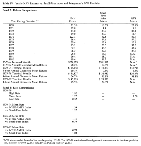
Table IV is reproduced below:
Below we have adapted the data from Table IV and looked at the performance in both absolute and relative terms to the S&P 500 Total Return (TR, i.e. including dividends):
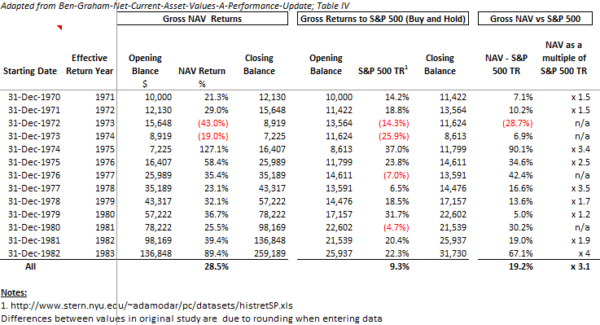
The results are hypothetical results and are NOT an indicator of future results and do NOT represent returns that any investor actually attained. Indexes are unmanaged and do not reflect management or trading fees, and one cannot invest directly in an index
Gross returns:
- Compound Annual Growth Rate (CAGR) of 28.5% (with rounding impacting our calculations) vs the S&P 500 TR 9.3%; an absolute outperformance of 19.2% and a multiple of 3.1 relative to the S&P 500 TR
- 1 losing year (1973, which incidentally also possessed the equal smallest sample size during the study period (18 securities; refer Table I, p 41.)
- 2 negative years vs 4 negative years for the S&P 500 TR
However, as Yogi Berra is claimed to have said,
“In theory there is no difference between theory and practice. In practice there is.” – Yogi Berra
Consequently, we simulated reality by adding commissions and taxes. We included commissions of 2% (1% to buy 1% to sell) and in relation to taxes, we utilized the capital gains taxes rates of the corresponding years(2) in the study and assumed our hypothetical investor resided in the US and sat in the highest marginal tax bracket but held on long enough to be eligible for the long-term capital gains tax rates. In contrast, we assumed an investor in the S&P 500 bought and held, never realizing their gains (and for simplicity we did not adjust their dividends for tax).
Net returns (i.e. including commissions and taxes):
- CAGR of 18.9% vs 9.3% for the S&P 500 TR; an absolute outperformance of 9.6% and a multiple of approximately 2 relative to the S&P 500 TR
- 4 losing years
- 2 negative years vs 4 negative years for the S&P 500 TR
In addition to commissions and taxes we also examined the impact of inflation(3), which was rampant during the period to ascertain its impact on returns.
Net Real returns (i.e. net of commissions, taxes and adjusted for inflation):
- CAGR of 10.7% vs 1.4% for the S&P 500 TR; an absolute outperformance of 9.3% and a multiple of 7.4 relative to the S&P 500 TR
- 4 losing years
- 2 negative years vs 5 negative years for the S&P 500 TR
Valuation Return Analysis
Table VI is reproduced from the study below:
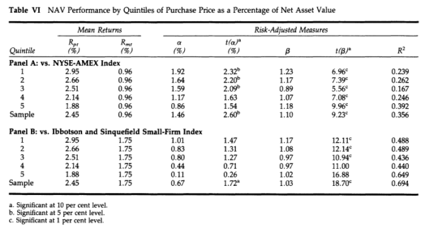
The results are hypothetical results and are NOT an indicator of future results and do NOT represent returns that any investor actually attained. Indexes are unmanaged and do not reflect management or trading fees, and one cannot invest directly in an index. Note: It is unstated whether this “mean monthly return” figure is intended to be a geometric or arithmetic mean. Oppenheimer “put[s] [the] results in a form more meaningful to an investor” by stating that “$10,000 invested in the NAV portfolio on December 31, 1970 would have grown to $254,973 (with monthly compounding) by December 31, 1983.” (p. 42.) However, that is a period of 156 months, and compounding $10,000 at 2.45% for 156 periods leads to a terminal value of $436,381, not $254,793. The implied compound monthly return rate for 156 periods and Oppenheimer’s terminal value is 2.10%. Consistent with this 2.10% figure, Oppenheimer states explicitly that the geometric mean annual return for the 13-year period was 28.2%. (p. 44.) Therefore, we conclude that the table above displays the arithmetic mean.
With regard to Table VI the author states;
“The conclusion is clear-cut. Returns and excess returns can be rank-ordered, with securities having the smallest purchase price as a percentage of net asset value having the largest returns. It appears that degree of undervaluation is important…”
Notwithstanding the above, due to concerns over the data used to measure returns (which is discussed in detail in subsequent sections), based on this study alone (and not taking into account our wider body of knowledge), the conclusion “that the degree of undervaluation is important” is not as reliable as it initially appears (despite its likely accuracy).
Earnings and Dividends
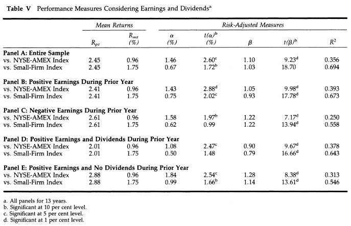
Table V is reproduced from the study below:
Dividends
When it comes to dividends the spread between “Positive Earnings and Dividends” (Panel D) and Positive Earnings and No Dividends (Panel E) is stark. No economic rationale comes to mind for why a net net paying dividends would underperform one that doesn’t pay dividends. Perhaps the spread is due to positive earning dividend payers possessing a shallower discount compared to positive earnings non-dividend payers. For instance, if positive earning dividend payers were consistently in the “most expensive” quintile (Table VI, Panel A) then their returns of 2.01% are similar to the 1.88% identified for the most expensive quintile. Similarly, if positive earning non-dividend payers were consistently in the “cheapest” quintile (Table VI, Panel A) then their returns of 2.88% are not materially different from the 2.95% identified for the cheapest quintile. That said, the aforementioned seems unlikely.
Interestingly in note 17 (p. 47) of the study the author specifies the following:
“An analysis of the 13 portfolios was also performed. The conclusions about earnings and dividends also hold for them” implying an element of robustness to the conclusion that “Firms having positive earnings and paying a dividend provided a lower mean return than portfolios of firms with positive earnings not paying a dividend. They also had a lower systematic risk. Finally, their risk-adjusted excess returns were not as high as those of the portfolio of firms with positive earnings but not paying dividends. Choosing only firms that have earnings and pay a dividend does not help the investor.”
It would appear then, that dividends, at least in relation to the period and market studied were a hindrance to returns…or were they?
Note 9 (p. 47) specifies the following:
“all comparisons with the exchange benchmarks returns without dividends are used for both the security return and the benchmark return.” Henry R. Oppenheimer
That is to say, to our understanding, the dividends have been excluded in the returns displayed in Table V (among others), therefore the returns have been artificially reduced by the amount of the dividend paid out. On this basis it isn’t at all unexpected that the dividend payers would seemingly underperform their non-dividend paying counterparts.
For clarity we will demonstrate using an example between a non-dividend and dividend-paying stock:
| Stock A (non-dividend) | Stock B (dividend) | |
| Price t0 | $10 | $10 |
| Price t1 | $13 | $12 |
| Price Return (excl. dividend) | $3 (i.e. 30%) | $2 (i.e. 20%) |
| Dividend | $0 | $3 |
| Total Return (incl. dividends) | $3 (i.e. 30%) | $5 (i.e. 50%) |
From the table above Stock B (the “dividend payer”) has produced the higher “total return” (i.e. 50% vs 30%), however, if you exclude the dividend Stock A (the “non-dividend payer”) appears to have produced the larger return (i.e. 30% vs 20%). While perplexing, it does, to our comprehension, appear as though this rudimentary error (i.e. excluding dividends) has been made in conducting this study.(4)
In light of the above, we are of the opinion that no reliable conclusion can be drawn in relation to the impact of dividends on the return to “net-nets” based on this study. Interestingly, it also means that returns of “net-nets” may be generally understated as a result of excluding dividends.
Earnings
The author sees the differential between “Positive Earnings” (Panel B) and “Negative Earnings” (Panel C) as marginal. The author concludes that:
“No clear-cut pattern emerges from an examination of these panels. If anything, firms operating at a loss seem to have slightly higher returns and risk than firms with positive earnings.” Henry R. Oppenheimer
However, in light of our findings with regard to the data used to measure returns (discussed in depth in the section titled “Dividends”) we deviate from the author’s assessment in relation to “positive” and “negative” earning net nets. We agree that “No clear-cut pattern emerges from an examination”; but do so for different reasons.
It is possible (probable in our view) that “positive earners” had a greater propensity to pay dividends. Therefore, if those dividends were not included in the measurement of their returns they would be artificially reduced. Of course, it is also possible (albeit unlikely in our view) that “negative earners” paid the greater share of dividends subsequently understating their returns. Irrespective, we are of the opinion that no reliable conclusion can be drawn in relation to the impact of earnings on the return of “net nets” based on this study.
Holding Periods, January effect, Size effect
Holding Periods
Table III is reproduced below:

While it would have been interesting to analyze the returns for portfolios held for 12 and 30 months this is not possible as the annual returns to the 12-month holding/rebalance period per Table IV are geometric means, whereas the returns displayed in Table III above are arithmetic means. However, the author’s commentary does specify that:
“The results largely parallel those of Table II” [which displays the monthly arithmetic mean for a 12-month holding/rebalance period]. From a return (and wealth) perspective, the advantage of the NAV portfolios over the market indexes is consistently pronounced.”
January effect
January effect; the author tested and found the return to the NAV portfolios
“while consistently smaller than those reported in Table III, still supported the conclusion that the NAV criterion provided satisfactory performance.” Henry R. Oppenheimer
That is to say, the performance of the NAV portfolios was not solely explained by the “January effect”.
Size effect
Size effect; to demonstrate that the returns to the NAV strategy were not merely a result of the “size effect” the author provides analyses (p. 45.) examining the return to the small-firm index and the “MV1” portfolio which is even smaller than the NAV portfolios. While we do not know the valuation of the small-firm index and the MV1 portfolio the conclusion that the returns to the NAV portfolios are not purely a result of the size effect seems reasonable.
However, no minimum market capitalization cut off for the securities examined in this study was mandated. Furthermore, we note that the reported median market capitalization of securities in the portfolios examined was 4.1m. That is to say, half the firms examined had a market capitalization equal to or below 4.1m which is particularly small, even by today’s inflation adjusted standards. The securities of the very smallest firms within a market are, in practice, virtually untradeable, even when attempting to deploy relatively modest amounts of capital.
In light of the foregoing it is highly probable that a considerable number of firms included in the study were, in effect, uninvestable. Consequently, the reported returns are highly likely to have been materially biased upwards given the findings reported in other research pertaining to the very smallest stocks within a market and their associated lack of liquidity(5).
Additional observations
One noteworthy comment that stands out from the study is as follows:
“Even though the NAV criterion is the valuation technique Graham is most famous for, it has been subject to relatively little research.’ Oppenheimer has provided tests of its performance over the 1949-72 period, but his tests (which do not demonstrate consistent profits) are largely confined to data prior to 1958.” (p. 40) Henry R. Oppenheimer
Interesting; unfortunately we have not found these other “tests”.
Conclusion
“Ben Graham’s Net Current Asset Values: A Performance Update” examined the performance of securities that were trading at no more than two-thirds of their “net current asset value (NAV)” during the 13 year period from 1970-82 period in the US. The study reported gross returns that were more than triple the returns of the S&P 500 TR. Our simulation determined that the aforementioned returns, on a net basis (i.e. after commissions and potential taxes) would have nearly doubled those generated by the S&P500 TR.
However, the study utilized data that excluded dividends (i.e. “price return” data as opposed to “total return” data) and therefore the conclusion reached in the study, “[c]hoosing only firms that have…. a dividend does not help the investor” does not appear to be reliable. Furthermore, as data excluding dividends was also used to measure the returns of “positive” and “negative” earning net-nets, no reliable conclusion can be reached in relation to the impact of earnings on the return of net-nets either(6). Critically, it is highly probable that the study included a considerable number of firms whose securities may have been too illiquid to actually trade. Moreover, the inclusion of such firms is highly likely to have biased the reported returns upwards.
While the study initially appeared to be reliable, in reality it suffered from a number of material flaws such that it is highly improbable that the reported returns could have been achieved by an investor in practice.
References[+]
| ↑1 | https://alphaarchitect.com/2015/04/01/where-to-find-cool-academic-finance-research/ |
|---|---|
| ↑2 | https://taxfoundation.org/federal-capital-gains-tax-collections-1954-2009/ |
| ↑3 | https://www.inflation.eu/inflation-rates/united-states/historic-inflation/cpi-inflation-united-states.aspx |
| ↑4 | While we attempted to contact Mr. Oppenheimer to attain clarification on the matter, unfortunately, he appears to have retired in 2016 (https://web.uri.edu/business/2016/02/10/professor-oppenheimer/) |
| ↑5 | James O’Shaughnessy, What Works on Wall Street: The Classic Guide to the Best-Performing Investment Strategies of All Time, 4th ed. Chapter 5 (New York: McGraw-Hill, 2011). |
| ↑6 | In and of itself the exclusion of dividends would have understated the reported returns |
About the Author: Gaurang Merani, CPA
—
Important Disclosures
For informational and educational purposes only and should not be construed as specific investment, accounting, legal, or tax advice. Certain information is deemed to be reliable, but its accuracy and completeness cannot be guaranteed. Third party information may become outdated or otherwise superseded without notice. Neither the Securities and Exchange Commission (SEC) nor any other federal or state agency has approved, determined the accuracy, or confirmed the adequacy of this article.
The views and opinions expressed herein are those of the author and do not necessarily reflect the views of Alpha Architect, its affiliates or its employees. Our full disclosures are available here. Definitions of common statistics used in our analysis are available here (towards the bottom).
Join thousands of other readers and subscribe to our blog.