In his book Stock Cycles: Why Stocks Won’t Beat Money Markets over the Next 20 Years(1), Michael Alexander (a research engineer at Pharmacia Corporation at the time of writing) conducted a 200-year study of the S&P 500 and its precursors. He posited that U.S. equities have alternated between secular bull and bear markets every 15-20 years.
By his computations, secular bull markets, on average, produced 12% annualized real returns across 200 years of market history (1800-2000). In stark contrast, secular bear markets averaged just 0% real returns over the same time period—i.e., secular bear markets tended to barely keep pace with inflation.
If we average the real returns across all secular bull and bear market regimes, we arrive at the commonly cited long-term annualized real return of U.S. equities—6%.(2)
But what is more fascinating about Alexander’s study is his claim that the causes of secular bull and bear markets alternate between the following four drivers:
- Low real earnings growth → secular bear
- High real earnings growth → secular bull
- High inflation → secular bear
- Disinflation → secular bull
He presents statistical evidence going back to the early 1800s, but for illustrative purposes here, we’ll start in the early 20th century:
- 1929-1949: Secular bear market driven by low real earnings growth. This was during the Great Depression when real earnings growth was negative from October 1929 until November 1948(3).
- 1949-1965: Secular bull market driven by high real earnings growth. In the aftermath of WWII, the U.S. was a manufacturing powerhouse, while the rest of the world was rebuilding. The real earnings growth during this period was over 3% annualized(4).
- 1965-1982: Secular bear market driven by high inflation. Recall the oil crisis of the 70s and bond yields near 20%. Earnings multiples on equities were in the single digits at the end of this period(5). CPI rose at an annualized rate of 6.5% over those 18 years.(6)
- 1982-2000: Secular bull market driven by disinflation. After Volcker squashed inflation, both equities and bonds entered into powerful bull markets. CPI grew at a much more reasonable 3.1% during this time period(7).
Alexander published his book in 2000, when the CAPE ratio on the S&P 500 was approximately 44(8). Thus, the 1982-2000 secular bull market was his final example. But from his framework, we can perhaps, in hindsight, extrapolate the following regimes:
- 2000-2009: Secular bear market driven by low real earnings growth. Recall that in both the dotcom bubble and the Great Financial Crisis, we saw S&P 500 earnings completely vaporize. In March 2000, the S&P 500 real earnings stood at $76.30 and by March of 2009, they had fallen to $8.27(9).
- 2009-2021(?): Secular bull market driven by high real earnings growth. The earnings growth from 2009 to year-end 2020 (even after the COVID recession) was greater than 23%(10).
If Alexander’s framework is correct—and we believe it might be worth considering—the next cycle would be a secular bear market driven by high inflation and that cycle may already be upon us(11).
What reasons do we have to believe we may be entering or have already entered a secular bear market driven by high inflation?
Here are a few:
- Negative Expected Equity Returns
- In 2000, when the U.S. equity market was transitioning into a secular bear market driven by low real earnings growth, the Aggregate Investor Allocation to Equities (AIAE) was forecasting -1% annualized returns over the ensuing 10 years. The actual annualized return for U.S. equities from 2000-2010 ended up being -0.2%.
- In 2009, when the U.S. equity market was presumably exiting the aforementioned secular bear market and entering the most recent secular bull market, the AIAE was forecasting returns of 15.8% annualized from 2009 to 2019. The market ended up delivering 16% annualized over that time period.
- At the most recent U.S. equity market peak in December 2021, the AIAE was forecasting slightly negative annualized returns for U.S. equities over the next 10 years (i.e., from 2021-2031). That is, at current levels, there does not appear to be much sustainable upside for U.S. equities over the next decade. This lack of sustainable upside seems much more likely to be associated with an impending secular bear market rather than with the continuation of the preceding secular bull market.
- The Last Shall Be First
- The premise of the long-term reversal factor is that assets that have strongly underperformed over the intermediate past (e.g., 5 years or more), tend to outperform going forward. So, let’s ask ourselves, “Which assets have underperformed over the last decade?” Precisely the ones we would expect to outperform in a high inflation environment—namely, energy stocks, materials stocks, commodities, etc.
- Indeed, Russia, a country with substantial exposure to commodities, had a CAPE ratio of only 8 in 2018 (and low CAPE ratios have been associated with high future returns).
- Further, since the bottom of the COVID selloff on March 24th, 2020, energy stocks have delivered the highest total return of any of the 10 S&P 500 sectors.
- Actual High Inflation
- It goes without saying that in order for us to be in a secular bear market driven by high inflation, we should actually be observing high inflation! And we are. It’s the talk of the town. High inflation is showing up in the official statistics (7% year-over-year CPI in December 2021), as well as anecdotally. It’s caused the Federal Reserve to pivot from its stance of inflation being “transitory” to forecasting multiple rate hikes in 2022.
In addition to these solid pieces of evidence, we also have data from how institutions and individuals are positioning themselves in the derivatives markets. And the implication is sobering.
Evidence from Relative Sentiment Indicators
In a series of papers and blog articles (see here, here, and here), we introduced some methods for computing the relative sentiment between institutional and individual investors. Relative sentiment is a measure of how institutions are positioned in the market relative to individual investors.
When institutions are more relatively bullish than individuals, equity markets tend to rise. When institutions are more relatively bearish than individuals, equity markets tend to go sideways or down.
One particularly interesting aspect of the research is that relative sentiment appears to provide more information than time-series momentum when it comes to forecasting future equity returns.
For example, when equity momentum is negative (e.g., equities are below their 200-day moving average or the 12-month return is negative), but institutions are relatively bullish, equities tend to have their best-annualized returns over the ensuing weeks and months. That is, “buy the dip” when equities have fallen, but institutions are bullish. In contrast, when equity momentum is positive, but institutions are relatively bearish, equities tend to go sideways rather than up (as positive momentum would otherwise suggest).
One of the aforementioned relative sentiment indicators, which we dubbed the “Smart Money Indicator” or SMI (because institutions are often thought of as the smart money), has recently provided evidence that further strengthens the case we may have already entered into a secular bear market driven by high inflation.
As a primer, the SMI looks at Commitments of Traders data and quantifies how institutions are positioned relative to individuals in equities, in long-duration bonds, and along the yield curve.
In particular, the SMI components include:
- A. The M-week maximum of the N-week z-score of institutions’ net percent of open interest in equities
- B. The M-week maximum of the N-week z-score of individuals’ net percent of open interest in equities
- C. The M-week minimum of the N-week z-score of institutions’ net percent of open interest in the long bond (both Treasury and Ultra Treasury bond futures)
- D. The M-week minimum of the N-week z-score of individuals’ net percent of open interest in the long bond (both Treasury and Ultra Treasury bond futures)
- E. The M-week maximum of the N-week z-score of institutions’ net percent of open interest in the 10Y bond (both the 10Y and Ultra 10Y)
- F. The M-week maximum of the N-week z-score of individuals’ net percent of open interest in the 10Y bond (both the 10Y and Ultra 10Y)
- G. The M-week maximum of the N-week z-score of institutions’ net percent of open interest in the long bond (both Treasury and Ultra Treasury bond futures)
- H. The M-week maximum of the N-week z-score of individuals’ net percent of open interest in the long bond (both Treasury and Ultra Treasury bond futures)
It then computes the following composite z-score from the above quantities:
composite z-score = 0.5 x [(A – B) – (C – D) + (E – F) – (G – H)]
Finally, the SMI is found by subtracting the cumulative median from the composite z-score.
SMI = composite z-score – cumulative median of composite z-score
If the SMI is greater (less) than 0, we consider institutions to be more relatively bullish (bearish) than individual investors.
The SMI rests on three assumptions:
- If institutions are more relatively bullish on equities, that’s bullish for equities
- If institutions are more relatively bearish on the long bond, that’s bullish for equities (hence the term “– (C – D)” in the equation above)
- If institutions are more relatively bullish the 10Y bond than the long bond, that’s bullish for equities (hence the terms “+ (E – F) – (G – H)” in the equation above)
Assumption 1 seems pretty straightforward given the fact institutions tend to have better outcomes in the financial markets than individuals. Hence, if institutions are more bullish on equities relative to individuals, that’s likely to be a bullish tailwind pushing equities higher.
But what about assumptions 2 and 3? They both derive from the fact that, over the time period of the SMI analysis (mid-to-late 90s to the present), the correlation between equities and the long bond has been negative. Thus, if institutions are expecting the long bond to fall, that’s almost akin to expecting equities to rise. Similarly, if institutions are expecting shorter-duration bonds (such as the 10Y) to outperform longer-duration bonds (such as the 30Y), that too might suggest equities are likely to rise.
This formulation of the SMI when applied to the equity markets from the 90s to the bottom of the pandemic selloff yielded the following results:
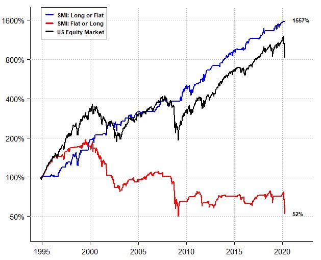
Figure 1. This figure plots the total return of the U.S. equity market (black), the total return from being long the U.S. equity market when the SMI (N = 52, M = 7) is greater than 0 and flat otherwise (blue), and the total return from being flat the U.S. equity market when the SMI is greater than 0 and long otherwise (red). Transaction costs and slippage are not considered.
But recent events have caused us to revisit assumptions 2 and 3—and what we have found is somewhat sobering for equity markets(12).
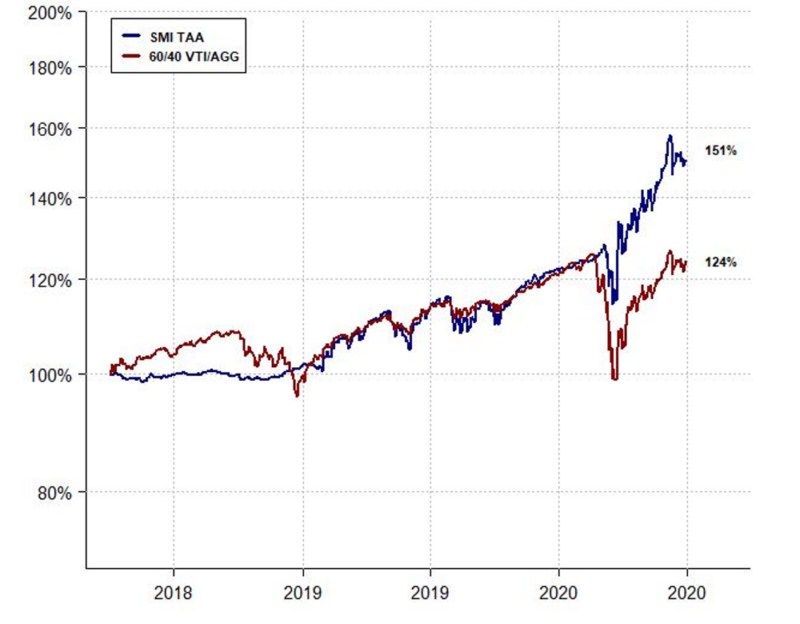
If we use the original SMI formulation and include the S&P 500 Stock Index, the S&P 500 E-mini Index, and the Nasdaq E-mini Index for our equity component, and include both the Treasury Bond and Ultra Treasury Bond for our long-duration component, and include the 10Y Bond and Ultra 10Y Bond for our shorter-duration component, the post-publication performance of the indicator from April 2018 through June 2020 is given in the chart below.
The (tactical asset allocation(13) version of the) SMI exited the equity market before the Q4 2018 selloff and also exited the market in December 2019 before the pandemic selloff began in late February. It then got max long the equity market on March 20th, 2020, two trading days before market bottomed. So far, so good.
The results are hypothetical results and are NOT an indicator of future results and do NOT represent returns that any investor actually attained. Indexes are unmanaged, do not reflect management or trading fees, and one cannot invest directly in an index.
But then the original-formulation SMI exited equities in June of 2020 with the S&P 500 around 3200. (We tweeted about this in real-time.) It then proceeded to sit on the sidelines (in bonds) as the S&P continued rallying up to 4200.
It then got long again in mid-2021 as the market proceeded to rally up near 4800 by year-end. The original-formulation SMI remains at a 100% allocation to equities, even as the market has fallen from all-time highs to around 4400, as of this writing (approximately an 8% drop).
In the grand scheme of things, an 8% drawdown for a tactical allocation strategy is nothing to get overly worked up about. But what caused us to rethink the SMI’s underlying assumptions is that all of the other relative sentiment indicators we use have significantly reduced their equity allocations in recent weeks.
If we average the desired equity exposure of those other relative sentiment indicators, we get a 33% target allocation to equities (and when we add in the original-formulation SMI’s 100% allocation, the overall average becomes 57% equities).
This disparity between the other indicators and the SMI was the penny that dropped.
The Correlation Regime Seems to Have Shifted
Over the time period from 1965 to 1982, when the U.S. equity market was in a secular bear market driven by high inflation, the correlation between monthly equity and long bond returns was positive (at approximately 0.35)(14).
From 1982 until the top of the dotcom bubble on March 24th, 2000, during which time the market was in a secular bull regime driven by disinflation, the correlation between monthly equity and long bond returns remained positive (at approximately 0.33, i.e., little changed from the prior bear market cycle)(15) .
From the top of the dotcom bubble (March 24th, 2000) to the bottom of the COVID panic (March 24th, 2020), the correlation between monthly equity and long bond returns was negative (at approximately -0.31)(16) . This period encompassed both a secular bear market and a secular bull market, each driven by the trajectory of real earnings growth.
Since the bottom of the COVID selloff through year-end 2021, the correlation between monthly equity and long bond returns has again been positive (at approximately 0.25)(17).
Thus, a plausible hypothesis might be that during secular regimes driven by inflation (or disinflation), when inflation eases (surges), long bonds and equity markets rejoice (despair) and rise (fall) somewhat in tandem.
In contrast, during secular regimes driven by real earnings growth—when inflation is not a problem— long bonds rise, and equities fall, on any whiffs of contraction; whereas any whiffs of growth cause the opposite to happen.
Positioning Correlations Have Also Shifted
Not only has the correlation between equity and long bond returns flipped sign, but the correlations between investor positioning and market returns have also reversed.
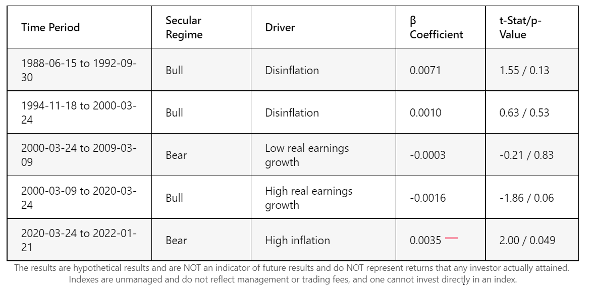
We ran regressions of weekly equity market returns against the prior end-of-week components of the SMI (shown above). In particular, we performed the following regressions:
a. Rmarket= α + β * (C-D) + ε
b. Rmarket= α + β * ((E-F) – (G- H)) + ε
We test both the long bond component, (C – D), and yield curve component, ((E – F) – (G – H)), of the SMI.
We ran each of these regressions over the following time periods:
- Secular Bull Driven by High Inflation: 1988-06-15 – 1992-09-30
- Secular Bull Driven by High Inflation: 1994-11-18 – March 24, 2000
- Secular Bear Driven by Low Real Earnings Growth: March 24, 2000 – March 9, 2009
- Secular Bull Driven by High Real Earnings Growth: March 9, 2009 – March 24, 2020
- Secular Bear Driven by High Inflation (Conjectured): March 24, 2020 – January 21, 2022
Prior to October 1992, the Commitments of Traders data was released biweekly; hence the first regression corresponds to biweekly returns and biweekly SMI components. The other regressions use weekly returns and weekly SMI components. The SMI parameters N and M were set to 52 and 7, respectively.
We are interested in the sign of the beta coefficient. We hypothesize that in regimes driven by inflation (i.e., regressions 1, 2, and 5), the sign will be positive, and in regimes not driven by inflation, the sign will be negative.
This is indeed what we found. The results are shown in the tables below. While not all the coefficients were by-the-book statistically significant, the signs were as expected. And for the most recent period, i.e., since the March 2020 low, the beta coefficients of the two regressions were significant.
Table 1: This table shows the results of the regression: Rmarket= α + β * (C-D) + ε, where (C – D) is the long bond component of the SMI formulation (C represents institutional positioning and D, retail traders’ positioning). We conjecture that during secular regimes driven by inflation, the β coefficient should be positive.
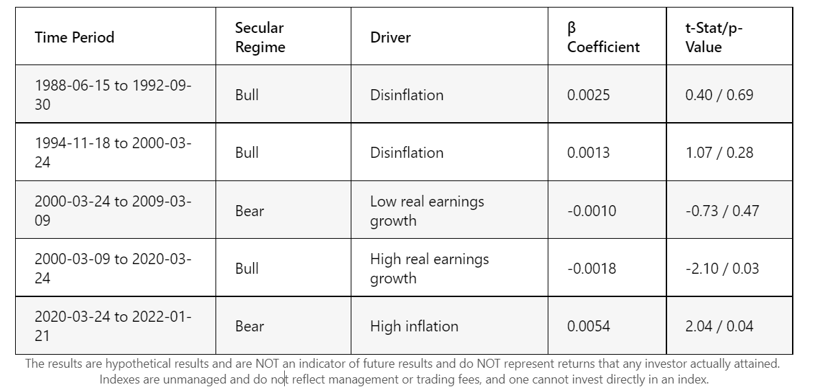
Table 2. This table shows the results of the regression: Rmarket= α + β * ((E-F) – (G- H)) + ε , where ((E – F) – (G – H)) is the yield curve component of the SMI formulation. We conjecture that during secular regimes driven by inflation, the β coefficient should be positive.
Regime-Adjusted SMI
In light of these findings, we propose a regime-adjusted SMI—one that attempts to identify the prevailing secular regime and modify the signs of the SMI’s components accordingly.
Thus, if we take the most recent beta coefficients into account and accept that we are in a secular bear market driven by high inflation, that would suggest we should calculate the SMI in the following way:
SMI = (A – B) + (C – D) – ((E – F) – (G – H)) – cumulative median of foregoing term
where the signs have been changed on the (C – D) and ((E – F) – (G – H)) terms. If we do this, the current desired equity allocation for the regime-adjusted SMI would be 0% and the strength of that signal would be substantial—almost -5 standard deviations! [Note: This calculation involves averaging over various parameter cases for N and M.]
Moreover, using a regime-adjusted SMI since the March 2020 low would have produced results more in line with the historical performance of the SMI indicator. For example, instead of exiting equities in mid-June 2020, the regime-adjusted SMI (averaged over various parameter cases) would have remained long or partially long until mid-June of 2021, exiting when the S&P 500 was approximately 4250.
Lastly, a regime-adjusted SMI would put it in tune with the other relative sentiment indicators we track that have suddenly turned bearish in the last several weeks. (The chart below shows the desired equity allocations of our suite of relative sentiment indicators since the March 2020 bottom.)
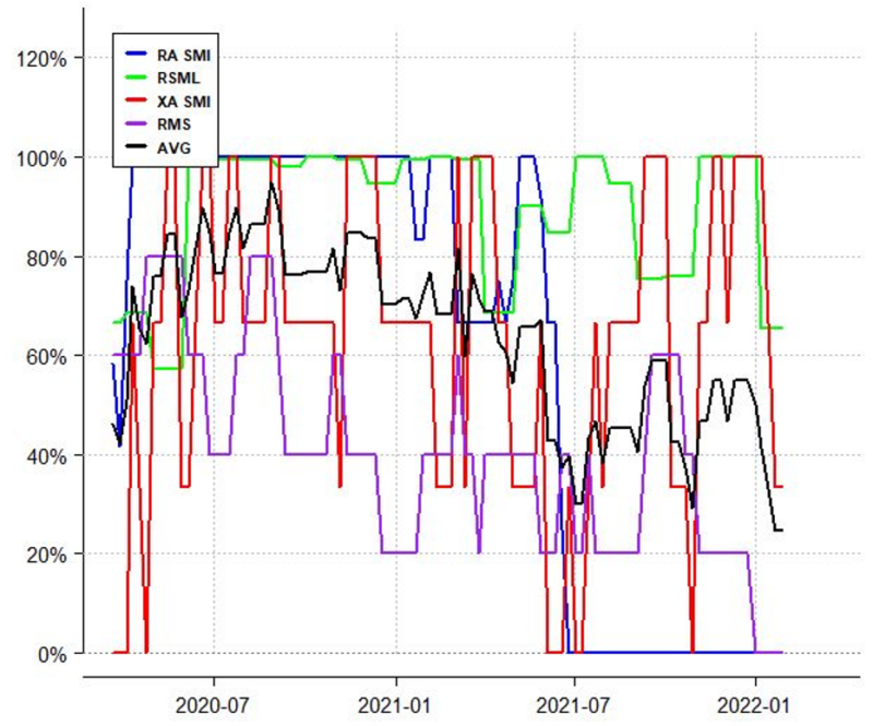
The results are hypothetical results and are NOT an indicator of future results and do NOT represent returns that any investor actually attained. Indexes are unmanaged, do not reflect management or trading fees, and one cannot invest directly in an index.
Somewhat concerningly, the overall average equity allocation derived from these four relative sentiment indicators would be approximately 25% if we were to factor in a regime-adjusted SMI. Such a reading is well below the historical average. When relative sentiment is bearish and equity momentum is negative, equities tend not to do well going forward. That is, “buying the dip” has not been a good strategy during such times.
Thus, unless some exogenous event were to happen, such as the Federal Reserve backtracking on its rate-hike forecasts(18), the equity market might very well be in for more choppiness, if not an outright downside in the near term.
Conclusion
The weight of the evidence suggests we recently exited a secular bull market driven by high real earnings growth and have entered a secular bear market driven by high inflation.
Future expected equity returns are at levels last seen at the top of the dot-com bubble. Assets that one would expect to outperform during inflationary secular regimes have begun outperforming. And inflation itself is outright high—year-over-year inflation in December 2021 was higher than the annualized inflation from 1965-1982.
Moreover, and perhaps most tellingly, correlations between equity returns and long bond returns have become positive (at monthly horizons). This is the same type of behavior observed during previous secular periods of high inflation (1965-1982) as well as during secular periods of disinflation (1982-2000).
Similarly, the correlations between equity returns and the component z-scores of the SMI have also changed signs—from negative to positive—which is what their polarity was from 1988-2000 during the last secular cycle driven by inflation.
If we take this regime change into account when computing the SMI, we observe forecasting behavior since the pandemic is more in line with its behavior prior to the pandemic and also more in line with other relative sentiment indicators (that don’t rely on equity/bond dynamics to quantify relative sentiment).
The takeaway is that while investors have become highly conditioned to buy the dip, the current dip is occurring with relative sentiment significantly bearish (i.e., retail likes equities more than institutions). Historically, that has not been a great time to buy equities.
References[+]
| ↑1 | published at the apex of the dotcom bubble in 2000 |
|---|---|
| ↑2 | Which might be on the high end as an observation. |
| ↑3 | Based on data from Yale professor Robert Shiller’s online data. |
| ↑4 | Based on data from Yale professor Robert Shiller’s online data. |
| ↑5 | Based on data from Yale professor Robert Shiller’s online data. |
| ↑6 | Based on data from Yale professor Robert Shiller’s online data. |
| ↑7 | Based on data from Yale professor Robert Shiller’s online data. |
| ↑8 | Based on data from Yale professor Robert Shiller’s online data. |
| ↑9 | Based on data from Yale professor Robert Shiller’s online data . |
| ↑10 | Based on data from Yale professor Robert Shiller’s online data. |
| ↑11 | Side note: in 2009, when the Federal Reserve began Quantitative Easing, many people were calling for high, unconstrained inflation. Using Alexander’s framework as a guide, we wrote an article for SeekingAlpha explaining why high inflation wouldn’t take hold—it has held up reasonably well in the intervening years.) |
| ↑12 | Notably, after we had first published the SMI research, we received feedback from readers both on Twitter and in private messages that asked, presciently, what would happen to the SMI if the correlations between equities and bonds were to change. |
| ↑13 | Found here |
| ↑14 | Found using data from Professor Amit Goyal’s website. |
| ↑15 | Found using data from Professor Amit Goyal’s website. |
| ↑16 | Found using data from Professor Amit Goyal’s website. |
| ↑17 | Found using monthly returns of VTI and TLT. |
| ↑18 | The last time both momentum and the SMI were significantly negative was in Q4 2018, right before the Powell Pivot on rates. |
About the Author: Raymond Micaletti
—
Important Disclosures
For informational and educational purposes only and should not be construed as specific investment, accounting, legal, or tax advice. Certain information is deemed to be reliable, but its accuracy and completeness cannot be guaranteed. Third party information may become outdated or otherwise superseded without notice. Neither the Securities and Exchange Commission (SEC) nor any other federal or state agency has approved, determined the accuracy, or confirmed the adequacy of this article.
The views and opinions expressed herein are those of the author and do not necessarily reflect the views of Alpha Architect, its affiliates or its employees. Our full disclosures are available here. Definitions of common statistics used in our analysis are available here (towards the bottom).
Join thousands of other readers and subscribe to our blog.