Albert Einstein is reported to have said the following:
The more I learn, the more I realize how much I don’t know.
We can relate.
Having studied finance for a long time (Ph.D., professor, books, articles, etc.), I think I now know less about how the stock market works.
In fact, I probably should have stopped studying finance after I read Ben Graham’s Intelligent Investor, over 20 years ago. Life would be a lot easier, or at least less complicated. Adhering to Graham’s straightforward value investing ethos certainly worked out for Warren Buffett:
What I’m doing today, at age 76, is running things through the same thought process I learned from the book [The Intelligent Investor] I read at 19.
And why should investing be complex, anyway? Asset pricing, or figuring out what something should be worth, seems easy in theory. And yet, when you review the vast swath of research dedicated to this question, there doesn’t seem to be any clear silver bullet answer.
Some might retort, “Valuation is easy,” figure out the expected cash flows and discount back to the present with an appropriate cost of capital, or “discount rate.”
Well, what’s the discount rate?
The discount rate is supposed to account for the risk of the expected cash flows, but what is the risk? How do we measure it?
Warren Buffet had this to say about the issue:
Charlie and I don’t know our cost of capital. It’s taught at business schools, but we’re skeptical…I’ve never seen a cost of capital calculation that made sense to me.
While the cost of capital is a notoriously imprecise valuation tool, there is still hope. Of the many ideas on the playing field, factor-based risk models seem to have captured the imagination of most empirical asset pricing researchers.(1)
But what is a factor-based model approach?
We answer this question — and many related questions — throughout this post.(2)
A PDF version of this is available here.
Jim Cramer Factor Investing: An Illustration
The factor approach has roots in what is deemed the arbitrage pricing theory, or APT.(3) Researchers seek to identify a set of factors (e.g., value, momentum, size, market, quality, low-vol, and so forth) that explain the so-called “cross-section” of returns, or the distribution of returns at a given point in time.
A simple example can clarify the concept. Let’s assume that the decibel level of Jim Cramer’s voice on CNBC is a proxy for systematic risk in the economy. So a stock that moves stronger when Jim Cramer is louder corresponds to more systematic risk, and should, therefore, require higher expected returns (i.e., more risk should equal more reward).
The simple relationship is outlined below.
Expected_Stock_return = risk_free_rate + B * Jim_Cramer_decible + randomness
Besides randomness and the baseline risk-free rate, the only thing that should drive expected performance is the exposure to the Jim_Cramer_decible factor. If a stock has a strong “beta” with respect to the Jim_Cramer_decible factor, then the expected stock return should be higher in the future, all else equal.
With this factor investing model in hand, we can now assess the risk and return associated with a stock by simply looking at the Jim_Cramer_Decibel risk factor exposure. If a stock earns high expected returns and has high Jim Cramer exposure — great — the model seems to work because it explains what happens in the real world. And if a stock earns low expected returns, and has low Jim Cramer exposure — great — again, the model seems to work. If a researcher conducts this analysis across a large sample of stocks, across a long sample period, and confirms the result through lots of robustness analysis, the model would be deemed the new Fama and French 1-Factor Cramer model in an academic paper.
Consultants would use it. Investors would use it. And the market efficiency world would be complete.
However, what if the Jim Cramer asset pricing model broke down?
Let’s say the model doesn’t always predict what happens in asset pricing markets. Perhaps we start seeing situations where the expected returns don’t match the risk profile; in other words, we see situations where stocks earn high expected returns but don’t have any measurable exposure to the Jim_Cramer_Decibel factor. The model no longer fits our observations. Oh no — Looks like we need a better model. Researchers will now scramble to identify a better model that explains why stocks act like they act. Maybe they’ll add new factors, delete old factors, and grind on regressions until the numbers sing.
Mission complete. Or is it?
The Jim_Cramer_Decibel risk factor identified above is obviously an attempt at finance humor (I know, pretty terrible. I get it). Nonetheless, the description of the process mirrors the basic approach serious academic researchers have used to identify factors that theoretically and empirically determine why stocks move, in expectation. And while the Jim Cramer decibel factor is tongue-in-cheek, some of the wilder explanatory “factors” that have been earnestly explored by reputable academics are not that far from it conceptually. In short, not all factors are created equal. Some factors are more reasonable than others.
The Original Factor Gangsta: The Capital Asset Pricing Model (CAPM)
One of the earliest attempts to explain how stocks move was posited in 1964, when Sharpe, Lintner and Black (SLB) developed their Capital Asset Pricing Model. The CAPM proposed something remarkable: all expected stock returns could be described via beta, which quantified the extent to which a stock return moved with the so-called market portfolio’s return (often approximated by a broad passive index, such as the S&P 500).(4)
Think about that — the CAPM suggests that ALL expected stock price movements revolve around a single, relatively simple, statistical metric. The elegance of the concept is arguably on par with E = mc 2 and the 1990 Nobel prize awarded to Markowitz and Sharpe(5) and was probably well deserved.(6)
Unfortunately, while the CAPM theory was beautiful, the evidence in support of the theory was flawed.(7) Academic research demonstrated that the relationship between beta and expected stock returns was too “flat”: Low-beta assets’ returns were higher than the risk-free rate, while high-beta assets showed returns that were lower than those suggested by the model. (Fama and French provide a good overview of the research).
The Figure below highlights the problem with the CAPM’s predictions versus reality:
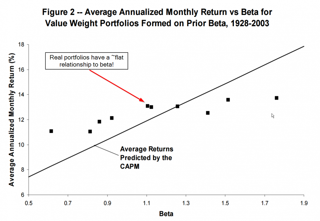
Note that real portfolios had a flat relationship with beta. In other words, knowing your beta didn’t tell you anything about expected returns. D’oh!
The CAPM was quickly dumped in the graveyard of great theories that don’t work in practice. Along came the CAPM apologists and new models with more factors that could help explain how and why stocks move. The primary puzzle to solve was why small-cap stocks and cheap “value” stocks were doing so much better than the CAPM predicted. On one hand, small-caps and value-stocks might reflect systematic mispricing (anti-efficient market hypothesis), but on the other hand, these styles of stocks may simply be riskier (pro-efficient market hypothesis). Fama and French came to the rescue…
Fama and French Lay the Foundation for Factor Investing
In response to the failure of the CAPM to explain the world, in 1992 Eugene Fama and Ken French, arguably the two greatest empirical financial economists of our time, established the empirical foundations for the Fama and French three-factor model, which did a much better job explaining anomalies, such as size and value.
The three-factor model included the original market factor from the CAPM, but added two new factors:
- A long/short size factor portfolio (small-minus-big, or SMB)
- A long/short value factor porfolio (high-minus-low, or HML)
Below is Table III from the original paper, covering the 1963-1990 period, highlighting the relationship between stock returns and beta (i.e., β), size (i.e., ln(ME)), and value (i.e., ln(BE/ME)) for NYSE, AMEX and NASDAQ stocks:
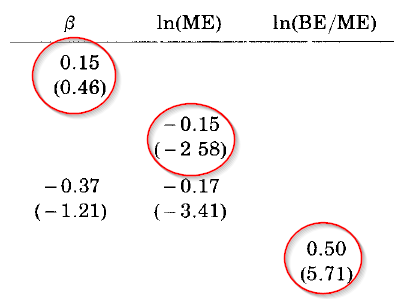
There are a few things to note.
- The slope of beta alone is 0.15% per month, with a t-statistic of 0.46. From this, Fama and French conclude that beta does not help explain average stock returns over the period. Fama and French described this as “a shot straight at the heart of the SLB model” (or CAPM).
- The slope for size (ln(ME)) is -0.15%, with a t-statistic of -2.58. Thus, Fama and French conclude that size has statistically significant explanatory power.
- The slope for value (ln(BE/ME)) is 0.50, with a t-statistic of 5.71. This suggests a very statistically strong relationship between returns and book-to-market equity.
Here is a visualization that highlights how poorly the CAPM predicted returns when portfolios are sorted on size and value. The chart plots excess returns against beta. The blue dots reflect realized returns associated with the so-called “Fama and French 25 portfolios,” which sort stocks into portfolios based on value and size (details are here). The red dots plot the CAPM predicted portfolio returns, had these portfolios earned their theoretically predicted premiums.
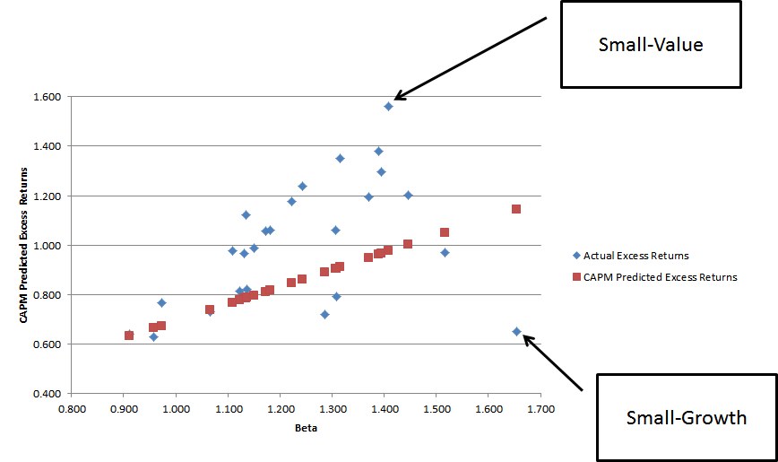
Note that the portfolios don’t line up very nicely along the CAPM predicted red dots. The relationship is really screwed up for small-cap value (earn way too much) and small-cap growth stocks (earn way too little).(8) The Fama and French 3 factor model rescued factor investing from the graveyard and helped researchers understand what characteristics drove stock returns.
Wait a minute: Active managers have alpha when we use the FF 3-factor model!
As factor analysis became more commonplace, thanks to the illuminating analysis from Fama and French 1992 and 1993, academics now had a tool to explain stock return movements. Researchers decided to apply these enhanced tools to explain mutual fund manager performance. Unfortunately, the early results concluded that mutual funds had persistent performance — winners kept winning and losers kept losing. These results also suggest that active managers may exhibit some level of skill.
But if active managers exhibit skill, this might imply markets aren’t efficiently pricing risk, which means markets aren’t efficient. Uh-oh!
In order to fix this problem, the research literature came up with a solution: when a factor investing model doesn’t work, simply add more factors.
In 1997, Mark Carhart followed the academic factor research modus operandi and created a new “four-factor model.” Carhart added a momentum factor (2-12 momentum, or “PR1YR,” also referred to as “UMD” or “MOM” depending on the researcher) to the Fama and French three-factor model, which significantly enhanced the explanatory power of the original model. Below is table II from the original paper, which sets forth performance statistics from 1963 to 1993:

In Carhart’s new four-factor model, SMB, HML, and PR1YR (momentum) had high mean average excess returns. Also, the factors have high variance and low correlation, which suggests they might do a good job in jointly explaining variation in stock returns and mutual fund manager performance.
Carhart applies his new factor model in the context of understanding mutual fund manager performance persistence. The key results from Carhart’s paper are highlighted in the graphic below (Figure 2 from the original paper). The past mutual fund winners (decile 1) seem to win in the future, but the reversion to the mean is strong and hard to distinguish from the other groups. However, if you are a past loser (decile 10), you tend to be a loser in the future.
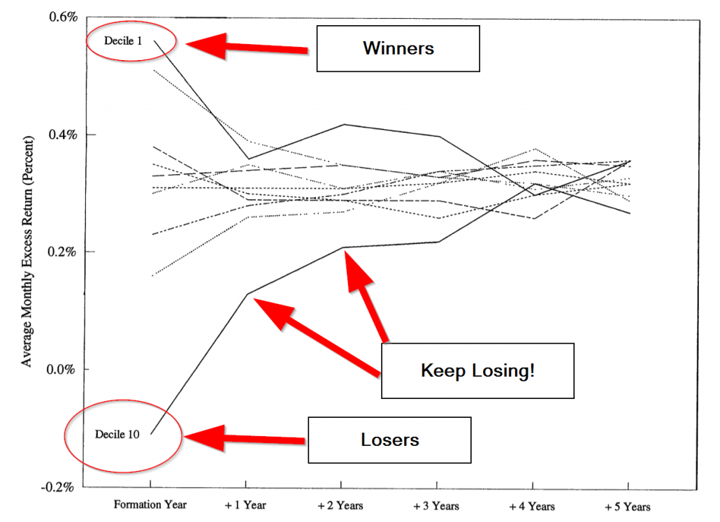
Carhart identifies some fascinating insights. Carhart highlights that winning active managers don’t win because they are skilled at identifying stocks that outperform, but rather, “Some mutual funds just happen by chance to hold relatively larger positions in last year’s winning stocks.” In short, winning mutual fund managers were momentum investors and didn’t even know it. And because the winning managers didn’t really know they won because of momentum exposure, we can’t attribute their performance to their skill (convoluted argument, I know!).
The takeaway from Carhart’s “momentum” factor is clear with respect to understanding mutual fund manager performance but muddied with respect to how we can think about his 4-factor model in the context of using it to understand stock returns. In fact, Carhart highlights in his paper that the inclusion of momentum in his 4-factor model is confusing. On the one hand, his model could be interpreted as a “risk” attribution model that suggests high performance is due to exposure to higher risk, which is proxied by exposures to beta, size, value, and momentum. However, on the other hand, his 4-factor model could also be viewed as a performance attribution model, which doesn’t make the claim that size, value, and momentum reflect risk factors (i.e., maybe they are “mispricing” factors), but rather, these factors simply do a good job of explaining performance.
Carhart’s paper leaves readers with a nagging question: Are factor models capturing risk exposures or mispricing effects?
Carhart’s momentum factor really opened up the discussion on the so-called “factor wars.” Momentum, or investing based on past prices, went directly to the heart of the weakest form of the efficient market hypothesis. Clearly, researchers needed to head back to the drawing board. One could not simply add more factors and claim a victory that the market was efficient, without identifying why the factors explaining the performance reflected a genuine risk premium. In other words, factor models can’t reflect a game of throwing spaghetti against the wall and seeing what sticks. Economists needed to better understand why factors matter.
Less Data-Mining and More Economic Theory
The three- and four-factor models ran the show for over a decade following their respective publications. Within academia, Fama and French and Carhart’s factor models were generally considered to be part of the empirical asset pricing discipline. However, critics were concerned that data-dredging drove the discipline and whatever results that had the highest t-stats won the day. At some level, there was nothing wrong with this approach — understanding the historical facts can be an important baseline for our understanding of how the world works (the core innovation from Fama and French 1992).
But correlation doesn’t help us fully understand causation.
The three-factor model was a perfect example of the problem. Sure, the model was great at explaining stock market movements, but what were the theoretical underpinnings as to why size and value characteristics determined expected returns? Size might be understandable — smaller stocks are less liquid, potentially have more business risk, etc. But value was more controversial — were these stocks actually riskier? Or were they simply suffering from mispricing as described by Ben Graham?
The financial economics profession was suffering and needed answers. First, their cherished CAPM model, which was elegant and grounded in rational economic theory, was no longer believable on empirical grounds. And now there were the three- and four-factor models highlighting that the stock market is more confusing than originally thought. Asset pricing theorists needed to take on the challenge of putting more rigor around factor models to try understand why, for example, size and value, were able to describe stock market movements.
The natural itch to have a sound theory behind multi-factor models needed to be scratched. Luckily, neoclassical economic theories, in particular the “q-theory of investment,” as advanced by James Tobin in the 1960s, explored a fundamentals-based approach to reconciling market prices with investment in corporate assets. In 2007, a paper by Lu Zhang and Long Chen, entitled “Neoclassical factors,” offered hints that a new combination of factors, based on “investment” and “profitability,” might explain returns better than the early ad-hoc factor models and, importantly, its theoretical basis drew from a different branch of financial economics–corporate finance, not asset pricing. Lu Zhang and colleagues continued their research trying to build a unified asset pricing theory that established economic logic behind a factor model. He set out on a stream of articles that hit on the same theme, but changed titles over time:(9)
- Neoclassical factors (July 2007)
- An Equilibrium three-factor model (January 2009)
- Production-based factors (April 2009)
- A better three-factor model that explains more anomalies (June 2009)
- An alternative three-factor model (April 2010, April 2011)
- Digesting anomalies: An investment approach (October 2012, August 2014)
As these new neoclassical “q factors” were further refined, it became clear that they offered a powerful alternative explanation for the cross-section of returns. Unfortunately, the powers that ran the top-tier academic journals were not interested in rocking the Fama and French 3-factor boat and Prof. Zhang and his colleagues had a challenging time getting their ideas published. But this situation would change when Fama and French decided to embrace the idea of creating an enhanced factor model with ties to economic theory.
Fama and French Adapt to New Research Findings
Perhaps seeing the handwriting on the wall that the three-factor model rested on a shaky theoretical foundation, Fama and French offered an enhancement to their three-factor model, in hopes of heading off competition from the q-factor concept developed by Zhang and others. By 2014, the dynamic Fama and French duo extended their model to include five factors, by adding two additional factors:
- Operating profitability (robust-minus-weak, or RMW), which is measured as revenues – COGS – SGA – interest expense, scaled by book value (t-1)
- Investment (conservative-minus-aggressive, or CMA), which is measured as YoY asset growth, scaled by total assets (t-1)
For those paying attention, these appeared to be thematically similar to the new q-factors proposed by Zhang et al.:
- Operating profitability ~ “ROE,” which is net income divided by lagged book value (very similar to Fama and French)
- Investment ~ “real investment factor,” which is the same YoY asset growth scaled by lagged total assets (the same as Fama and French)
Had Zhang & Co. been cut off at the academic pass by Fama and French? We will never know. Nonetheless, Hou, Xue, and Zhang ran a horse race on the competing factor models with a keen eye on the performance between their Q-factor model and the new Fama and French 5-factor model (covered briefly here).
The abstract from the Hou, Xue, and Zhang paper says it all:
This paper conducts a gigantic replication study of asset pricing anomalies by compiling an extensive data library with 437 variables… the q-factor model and a closely related five-factor model are the two best performing models among a long list of models. Investment and profitability are the dominating driving forces in the broad cross section of average stock returns.
Here is the key table from the paper:
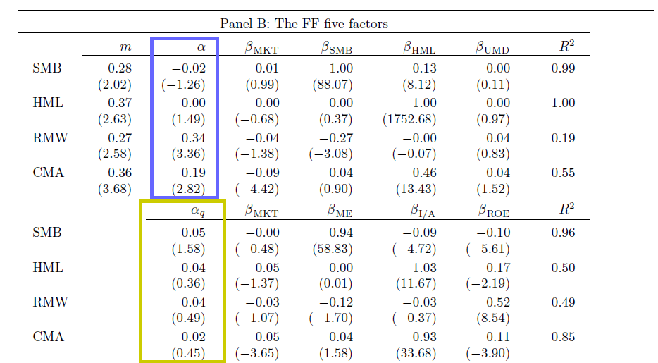
The Hou, Xue, and Zhang 4-factor model captures all the returns associated with the new 5-factor model outlined by Fama and French. Note the alpha estimates above. The yellow box highlights the alphas associated with the Fama and French factors, controlling for the Hou, Xue, and Zhang 4 factors and the blue box highlights the alphas associated with the Hou, Xue, and Zhang factors, controlling for the FF 5 factors. The Hou, Xue, and Zhang factors do a good job explaining the Fama and French factors (there are no statistically significant intercepts), but the Fama and French factors cannot explain the Hou, Xue, and Zhang factors. This suggests that Fama and French’s “new” profitability factor may not be a new dimension at all, since it can be explained quite well via exposures to the market, size, and Hou, Xue, and Zhang’s investment and ROE factors.
Interestingly enough, while the two research teams debated the merits of their respective models, one fact stood out: both researchers found that the value effect may not be real!
How can this be? Value had always been part of the factor literature! The new factor research suggested that value was simply a proxy for risk exposures to profitability and investment factors. And once you control for the new profitability and investment exposures, value ceased to have explanatory power. In short, value was dead.
The comments below, taken directly from source papers, describe their findings:
First, Fama and French highlight that value is dead:
With the addition of profitability and investment factors, the value factor of the Fama and French three-factor model becomes redundant for describing average returns in the sample we examine.
Hou, Xue, and Zhang take things a step further and suggest that both value and momentum are dead:(10)
The alphas of HML and UMD [momentum] in the q-factor model are small and insignificant, but the alphas of the investment and ROE factors in the Carhart model (that augments the Fama and French model with UMD) are large and significant. As such, HML and UMD might be noisy versions of the q-factors.
Step Aside Ivory Tower: Practitioners Offer Their Opinion
At this point, the argument over the king of factor investing models was limited to the domain of uber-geeks like Fama and French, and the Hou, Xue, and Zhang team. The Hou, Xue, and Zhang model is arguably better on both empirical and theoretical grounds. Of course, outside of academic researcher circles, practitioners started to add their 2 cents. For example, a newer paper from a joint team of academics and researchers at Robeco Asset Management, aptly named, “Five Concerns with the Five-Factor Model,” goes straight to the heart of these models.
Here is the abridged abstract:
…Although the 5-factor model exhibits significantly improved explanatory power, we identify five concerns with regard to the new model. First, it maintains the CAPM relation between market beta and return…Second, it continues to ignore the…momentum effect. Third, there are a number of robustness concerns…Fourth…the economic rationale for the two new factors is much less clear…Fifth…it does not seem likely that the 5-factor model is going to settle the main asset pricing debates…
And of course, there isn’t a real factor debate unless Cliff Asness and his team at AQR weigh in. Asness was struck by the reported redundancy of the so-called “value” factor, or “HML” factor, described in Fama and French and Hou, Xue, and Zhang. He decided to investigate the issue on his own in his article, “Our Model Goes to Six and Saves Value from Redundancy Along the Way.”
First, Cliff replicated Fama-French’s findings. Sure enough, they checked out. The evidence also highlighted that HML doesn’t matter once RMW (profitability factor) and CMA (investment factor) are included.
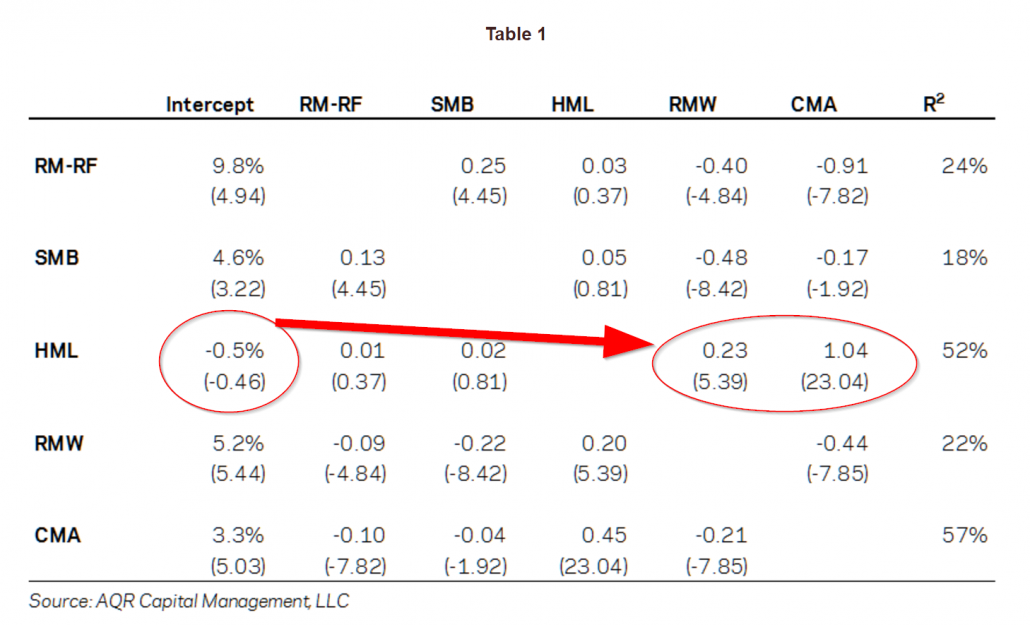
Next, he considered the elephant in the room that all factor models need to address, but rarely do: Momentum (described early in the Carhart discussion). In other words, Asness decided to see what would happen if he added momentum to the Fama and French 5-factor model, and created a six-factor model.(11)
Perhaps not surprisingly, Asness found that adding momentum enhanced the explanatory power of the model (strong t-stat of 4.11), however, value still seemed to be redundant (i.e., low t-stat or .51!)
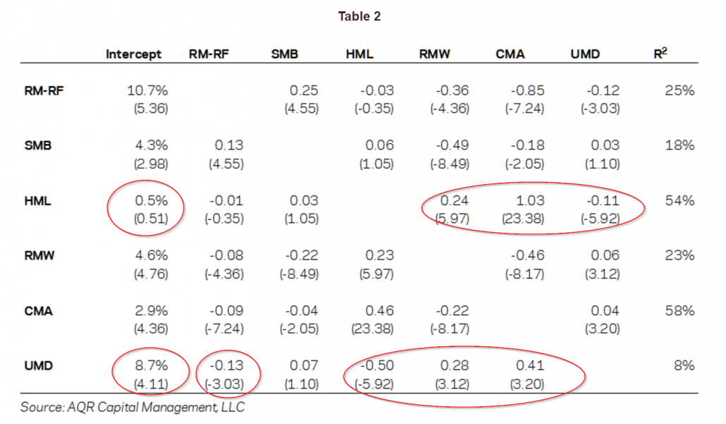
Was value simply a proxy for exposure to profitability and investment risk factors? That is what the evidence suggested, but Asness wasn’t done with his investigation.
Questioning the Value Factor’s (“HML”) Construction
Asness had some fundamental questions about what constituted “value”. He pointed out in a 2013 paper, “The Devil in HML’s Details,” that when Fama-French construct HML, they need two pieces of information:
- Book value of equity
- Price.
How do Fama and French calculate these?
- Book Value. Fama and French portfolios assume a six-month lag on book equity data, since sometimes it takes time for this accounting information to be disseminated into the market. The idea here is that this reduces the risk of “look-ahead” bias.
- Price. Fama and French portfolios also assume a six-month lag on price. The idea here is that the price matches the book value, so you are working with the actual book-to-price at a given date.
Why Fama and French went with this original construction is a bit odd: Why input a 6 month lag on price, when price would be readily known when the B/M portfolios are formed? .(12)
Sidestepping the reasons why Fama and French rationalized the use of lagged prices for sorting value portfolios — which seem to make no sense — Asness and Frazzini found that using a more realistic value sorting technique — with updated prices — created a more effective value premium
The Devil in HML’s Details Actually Matter
Asness re-ran his six-factor model (Fama and French 5-factor + momentum), and made two changes to HML:
- He used up-to-date price information
- He used a monthly rebalance.
The “new” HML factor is referred to as “HML-Devil.” The output from the regressions are below, covering 1963-2013:
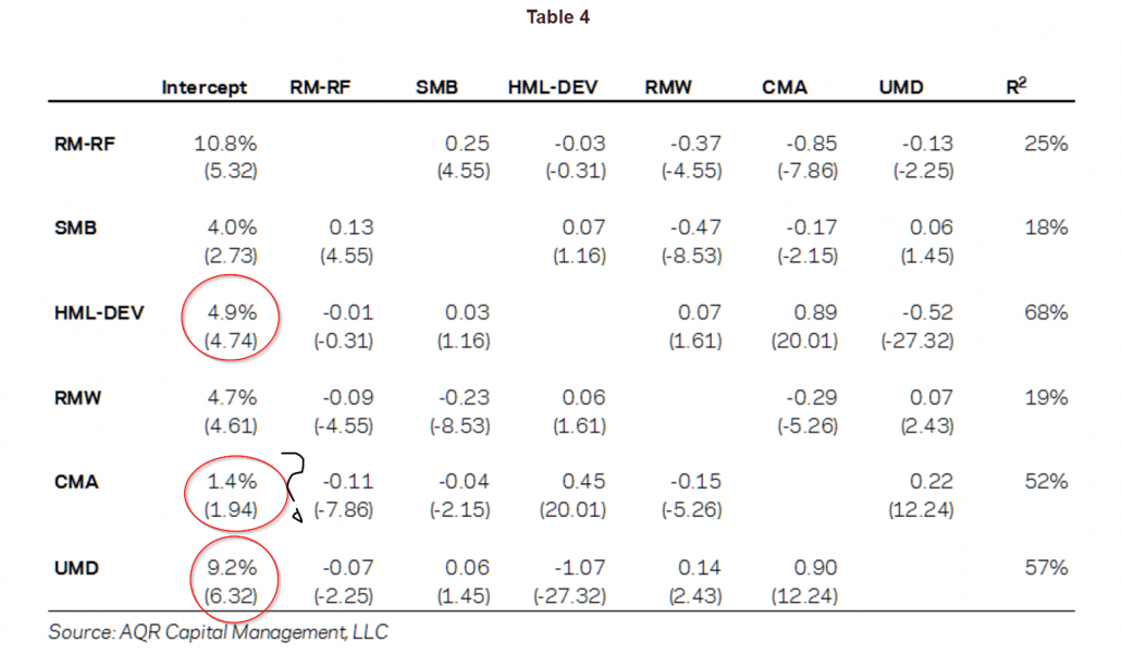
As Asness put it, “Shazam, shazam, shazam!” The HML factor was back and UMD (momentum) was even more powerful.(13)
Asness argues that the way Fama and French construct their HML factor diminishes the true relationship between value and momentum. After including a more pragmatic value factor, it is the investment factor (i.e., CMA) that becomes redundant — not the value factor — and now we have come full circle and are back to where we started — value and momentum are back as factor kings. But now we are faced with the original critique of the three-factor model: the empirical evidence is clear that value and momentum matter, but there are no rational economic theories that explain why! The q-theory approach was a commendable effort, but has holes and this raises questions about both the empirical design and theoretical foundations for the 5-factor model. D’oh! (14)
What Next? Factor Investing Wars Will Probably Last Forever
Hou, Xue, and Zhang moved the factor investing discussion to a higher level and took on the challenge of trying to tie factor models to a rational economic theory associated with investment decisions on behalf of firms. Their approach outlines the q-factor model, which uses two simple accounting variables, representing “investment” and “quality,” or ROE. The goal of their research was bold: Create a theoretically sound factor model that was empirically superior to ad-hoc factor models studied in the past. Their efforts are commendable and arguably influenced Fama and French to develop their new 5-factor.
But then the evidence happened. And behavioral-based explanations were never really ever considered.
Small changes on model design (e.g., HML_Devil versus HML, or the enterprise multiple factor, which we didn’t even cover!) allowed value and momentum anomalies to rear their ugly heads into the picture again. These tweaks also made the q-factor concepts (profitability and investment) less impressive and/or redundant. Other research on the subject also shows that profitability, for example, is not very robust. See here, here, and here. On the investment side, authors question the empirical validity of the finding. For example, Fangjian Fu finds that how one controls for delisting data can dramatically alter the empirical results associated with the “investment factor.” Also, Fama and French, who include investment as a factor in their 5-factor model, published a paper in 2008 that questions the robustness of the investment factor, suggesting that it is entirely driven by micro-cap stocks.
So despite the herculean mental efforts on behalf of academic researchers to better understand how stocks move, it seems that value and momentum still matter (as does size, beta, and profitability). But this truth doesn’t sit well with the mental models of many who study financial markets (i.e., the market efficiency crew).
Will we ever understand why factors exist? I think there is hope.
An alternative approach is to change the mental model for understanding the theoretical underpinnings for factor models. For example, in order to explain the value and momentum factors, one may need to wander beyond the realm of traditional rational economic theories. To understand these anomalies one may need to loosen theoretical constraints to encompass the view that 1) investors are irrational (behavior can be wack) and 2) frictional costs matter (limits of arbitrage). This train of thought is often referred to as behavioral finance. But relaxing the assumption that investors can be irrational, does not imply there is easy money lying around, which we explain here, however, relaxing these assumptions may help us better understand why risk/mispricing factors like value and momentum continue to “stick” in factor models.
Of course, relaxing rational constraints adds degrees of freedom for modelers and makes the challenge of understanding reality more difficult. Perhaps this trade-off is best outlined by Eugene Fama in his incredibly insightful piece, “Market Efficiency, Long-Term Returns, and Behavioral Finance.”
Here is the abstract from the paper:
Market efficiency survives the challenge from the literature on long-term return anomalies. Consistent with the market efficiency hypothesis that the anomalies are chance results, apparent over-reaction to information is about as common as under-reaction. And post-event continuation of pre-event abnormal returns is about as frequent as post-event reversal. Consistent with the market efficiency prediction that apparent anomalies can also be due to methodology, the anomalies are sensitive to the techniques used to measure them, and many disappear with reasonable changes in technique.
For fun, I did a thought experiment. What would happen if someone simply reversed the wording from Fama’s abstract and communicated the behavioral message:
Long-term return anomalies survive the challenge from the literature on market efficiency. Consistent with the market inefficiency hypothesis that instances of market efficiency are chance results, evidence that prices react appropriately to information are sparse. And evidence that post-event prices are efficient following pre-event information are few and far between. Consistent with the market inefficiency prediction that instances of market efficiency can also be due to methodology, evidence for market efficiency is sensitive to the techniques used to measure them, and much of this evidence disappears with reasonable changes in technique.
The “behavioral” version of Fama’s abstract could arguably stand as strong based on the collective evidence — if not stronger — than the statement put forth by Fama. (15)
I think Fama says it best in a recent 2016 interview with Joel Stern.
A few highlights from their conversation:
- After a half‐century of research and refinements, most asset‐pricing models have failed empirically.
- Estimating something as apparently simple as the cost of capital remains fraught with difficulty.
- The wide range of estimates for the market risk premium — anywhere from 2% to 10% — casts doubt on their reliability and practical usefulness.
Sure sounds to me like we are about as close to understanding the science of finance as we are to understanding the science of astrology. We’re probably better off understanding the insanity of investors and the incentives of delegated asset managers if we want to understand the science of investing, but this is controversial among many financial economists. We also probably want to understand firm investment decisions and their implications for expected returns (the “q-theory” route). Perhaps behavioral and rational ideas can both be used to better understand “why” things happen in markets? That seems like a reasonable approach, but because an integrated approach quickly dissolves into what essentially maps to a narrative, “proving” that a combination of behavioral and rational incentives drive stock markets is a tough — and probably impossible — task.
The painful reality is that factor investing will almost always be an art, and maybe a little bit of science…
Editor note: Thanks to Art Johnson, Andrew Miller, David Foulke, Jack Vogel, Doug Pugliese, Tadas Viskanta and many others for comments.
References[+]
| ↑1 | see our discussion of Berkin/Swedroe’s new book — Your Complete Guide to Factor-Based Investing. |
|---|---|
| ↑2 | David Foulke helped out a lot in drafting this post |
| ↑3 | Feel free to dig in for a deeper discussion, but we will not discuss the gory details here. |
| ↑4 | Technically, beta is calculated with respect to the excess market portfolio return (i.e., MKT – RF) |
| ↑5 | Merton Miller was in the mix as well |
| ↑6 | Here is a crash course on the concept, if you’d like to refresh. |
| ↑7 | Richard Roll argued that the theory is untestable, but that doesn’t really help us learn anything. |
| ↑8 | For those curious, we posted here about how to use the Fama and French model in practice. An in-depth discussion is available here. Finally, to examine some of these ideas in practice, we recommend Portfoliovisualizer. |
| ↑9 | source: Lu Zhang |
| ↑10 | others may disagree |
| ↑11 | Asness does not investigate the Hou, Xue, and Zhang model directly |
| ↑12 | I sometimes wear a t-shirt related to this finding around the office |
| ↑13 | This research doesn’t consider that HML, constructed using book-to-market, isn’t even the king of value factors. See our recent paper on the enterprise multiple factor. |
| ↑14 | A new paper that looks at the out of sample of the investment and profitability factors finds that profitability is robust, investment is not robust, and value still matters. |
| ↑15 | For example, Prof. Stambaugh, a stalwart of the efficient market hypothesis and thought leader in the space for decades, has even loosened his stance on the “old way” of viewing the world. See this paper as an example. |
About the Author: Wesley Gray, PhD
—
Important Disclosures
For informational and educational purposes only and should not be construed as specific investment, accounting, legal, or tax advice. Certain information is deemed to be reliable, but its accuracy and completeness cannot be guaranteed. Third party information may become outdated or otherwise superseded without notice. Neither the Securities and Exchange Commission (SEC) nor any other federal or state agency has approved, determined the accuracy, or confirmed the adequacy of this article.
The views and opinions expressed herein are those of the author and do not necessarily reflect the views of Alpha Architect, its affiliates or its employees. Our full disclosures are available here. Definitions of common statistics used in our analysis are available here (towards the bottom).
Join thousands of other readers and subscribe to our blog.


 https://alphaarchitect.com/wp-content/uploads/2016/12/hml-devil.png 737w" sizes="(max-width: 737px) 100vw, 737px" />