Editor’s Note: Valeriy Zakamulin is one of the world’s experts on trend following and technical trading rules and will be providing a multi-part series on the subject. This is part one in the technical series. Enjoy. (here is an old piece we have on Valeriy’s research)
—
One of the basic principles of technical analysis is that “prices move in trends.” Traders firmly believe that these trends can be identified in a timely manner and used to generate profits and limit losses. Consequently, trend following is arguably one of the most widespread market timing strategies; it tries to jump on a trend and ride it. Specifically, when stock prices are trending upward (downward), it’s time to buy (sell) the stock.
Even though trend following is a simple concept, implementation can get complicated. One of the major difficulties is that stock prices fluctuate wildly due to imbalances between supply and demand and due to constant arrival of new information about company fundamentals. These up-and-down fluctuations make it hard to identify turning points in a trend. Moving averages are used to “smooth” the stock price in order to highlight the underlying trend.
This methodology of detecting the trend by filtering the noise comes from time-series analysis, where centered (or two-sided) moving averages are used. It is common to think about the time-series of prices as comprising two components: a trend and “noise.” The idea is that noise represents short-term fluctuations around the trend. Therefore this noise can be removed by smoothing the data using a centered moving average.
Denote by {P1,P2,…,PT} a series of observations of the closing prices of a stock over some time interval. Any moving average of prices is calculated using a fixed size data “window” that is rolled through time. The length of this window of data, also called the averaging period (or the lookback period in a trailing moving average), is the time interval over which the moving average is computed. Denote by n the size of the averaging window which consists of a center and two halves of size k such that n=2k+1. The computation of the value of a centered moving average at time t is given by


When the noise is removed, the value of the trend component is then the value of the centered moving average. The size of the averaging window n is selected to effectively remove the noise in the time-series. In principle, the longer the size of the averaging window, the better a moving average removes the noise in a data series and the easier it is to detect turning points in the trend. Regardless of the size of the averaging window, the shape of a centered moving average follows closely the underlying trend in a data series and the turning points in a centered moving average coincide in time with turning points in the intrinsic trend.
So far, a centered moving average seems like a simple and effective tool that allows the trader to identify a price trend and find turning points in a trend. But there is a catch involved. Specifically, to compute the value of a centered moving average at time t, the trader needs to know the prices at subsequent times (t+1, …, t+k). Therefore, a centered moving average cannot be used to detect a trend and identify turning points in real time; it can only be used to analyze the past data.
At time t the trader knows only the stock prices until that time. Consequently, at t the trader can use only the available data to compute the value of a moving average. In this case the value of a (right-aligned) moving average at t is computed as


A comparison of the formulas for the calculation of the centered and right-aligned moving averages reveals that the value of the right-aligned moving average at time t equals the value of the centered moving average at time t-k


Thus, a right-aligned moving average represents a lagged version of the centered moving average computed using the same size of the averaging window. Therefore a right-aligned moving average has the same smoothing properties as those of a centered moving average. Specifically, the longer the size of the averaging window in a right-aligned moving average, the better a moving average removes the noise in a data series. However, the problem is that the longer the size of the averaging window, the longer the lag time.
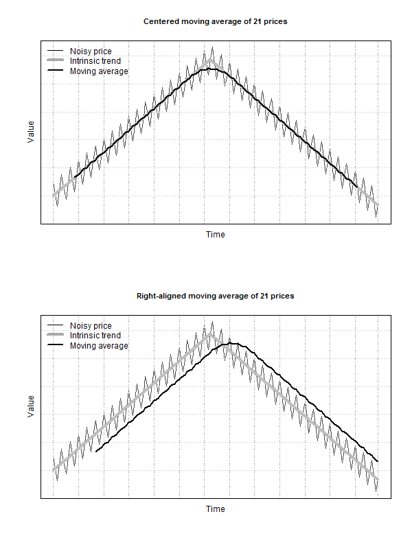
The properties of the centered and right-aligned moving averages are illustrated in figure below (see a similar interactive illustration). These illustrations are based on using artificial stock price data where the stock price trend is given by two linear segments. First, the stock price trends upward, then downward. We add noise to the trend and this noise is given by a high frequency sine wave. The goal of these illustrations is to visualize the shapes of a centered moving average and a right-aligned moving average and their locations relative to the (intrinsic) stock price trend.
The results are hypothetical results and are NOT an indicator of future results and do NOT represent returns that any investor actually attained. Indexes are unmanaged, do not reflect management or trading fees, and one cannot invest directly in an index. Additional information regarding the construction of these results is available upon request.
Both moving averages are computed using a window of 21 price observations. With this window size, both moving averages effectively remove the noise in the price. However, whereas the turning point in a centered moving average coincides in time with the turning point in the price trend, the turning point in a right-aligned moving average lags behind the turning point in the price trend. Therefore any right-aligned moving average represents a smoothing tool with a time lag. That is, all right-aligned moving averages used for the purpose of timing the market identify a turning point in a trend with a delay.
General Weighted Moving Average
In the preceding section we considered the simplest type of a moving average where equal weights are given to each price observation in the window of data. This section introduces the general weighted moving average computed using the averaging window of size n. In this window, each price observation has its own weight in the computation of a general moving average. Specifically, a general moving average at time t is computed using the last closing price Pt and n-1 lagged prices Pt-i:


where wi is the weight of price Pt-i in the computation of the weighted moving average. The set of weights is not normalized, meaning that the sum of weights is not equal to one. One can use instead the normalized weights


and compute the time t moving average as


The set of weights given by either {w0, w1,…,wn-1} or {ψ0, ψ1,…,ψn-1} is usually called a “weighting function.” Each specific type of a moving average has its own distinct weighting function.
Average Lag Time of a Moving Average
The weighting function of a moving average fully characterizes its properties and allows us to estimate the average lag time of the moving average. The idea behind the computation of the average lag time is to calculate the average “age” of the data included in the moving average. A similar idea is used in physics to compute the center of mass and in finance to compute the bond duration (Macaulay duration). In particular, the price observation at time t-i has weight wi in the calculation of a moving average and lags behind the most recent observation at time t by i periods. Consequently, the incremental delay from observation at t-i amounts to wi×i. The average lag time is the lag time at which all the weights can be considered to be “concentrated.”
The average lag time of a weighted moving average is computed using the following formula


The formula for the average lag time can be rewritten as (we skip the details of the derivation to save space)


where the weight φj is given by


Alternative Representation of a Moving Average
The formula for the weighted moving average (given by equation (1)) gives little insight into the properties of moving averages. We suggest an alternative and novel representation of a moving average. This alternative representation allows us to look at a moving average from a new perspective. In addition, this alternative representation allows us to reveal the properties of moving averages.
The alternative representation of a moving average is motivated by the fact that a series of stock prices can be considered as a dynamic process in time. We introduce the notation


which is the change in the stock price over the time interval from t-i to t-i+1. Using this notation, we can write


Therefore the formula for the weighted moving average can be rewritten as


Interchanging the order of summation in the double sum above yields


where φj is given by equation (5). Therefore, all (right-aligned) moving averages can be represented as the last closing price minus the weighted sum of the price changes in the averaging window. Typically, in a moving average the weights are positive, wi>0 (ψi>0) for all i. As a result, in this case the sequence of weights φj is positive and decreasing with increasing j


Consequently, regardless of the shape of the weighting function for prices wi, the weighting function φj always over-weights the most recent price changes. In the subsequent exposition, we will call the weighting function ψi (i≥0) the (normalized) “price weighting function” and the weighting function φj (j≥1) the (normalized) “price-change weighting function.”
Properties of Moving Averages
To understand the relationship between the stock price Pt and the value of the moving average MAt(n), let us rewrite equation (6) as


The following conclusions can be drawn from this equation:
- The value of a moving average equals the last closing price when the sum of the weighted price changes equals zero. For example, this happens when the price remains on the same level (that is, the price goes sideways) in the averaging window.
- When the prices move steadily upward such that ΔPt-j>0, then Pt-MAt(n)>0. That is, when the prices are in uptrend, the moving average tends to be below the last closing price.
- When the prices move steadily downward such that ΔPt-j<0, then Pt-MAt(n)<0. That is, when the prices are in downtrend, the moving average tends to be above the last closing price.
In finance it is common to perceive the stock price change as a random variable. The probability distribution of a random variable can be characterized by its moments: expectation, variance, etc.
Motivated by this observation, let us compute the expected difference between the last closing price and the value of the moving average:
![(7) \quad E\left[P_t-MA_t(n)\right] = E\left[\sum_{j=1}^{n-1} \phi_j \Delta P_{t-j}\right] = \sum_{j=1}^{n-1} \phi_j E[\Delta P_{t-j}] = \text{Lag time}(MA)\times E[\Delta P],](data:image/svg+xml,%3Csvg%20xmlns='http://www.w3.org/2000/svg'%20viewBox='0%200%20582%2052'%3E%3C/svg%3E "Rendered by QuickLaTeX.com")
![(7) \quad E\left[P_t-MA_t(n)\right] = E\left[\sum_{j=1}^{n-1} \phi_j \Delta P_{t-j}\right] = \sum_{j=1}^{n-1} \phi_j E[\Delta P_{t-j}] = \text{Lag time}(MA)\times E[\Delta P],](https://alphaarchitect.com/wp-content/ql-cache/quicklatex.com-9beffbe02e9ae009556cea8514fb0dbd_l3.png "Rendered by QuickLaTeX.com")
where E[ΔP] is the expected change in price and the last equality follows from equation (4). In words, the expected difference between the last closing price and the value of the moving average equals the average lag time times the average price change. Equation (7) is very insightful and implies the following properties:
- The longer the average lag time, the larger the expected discrepancy between the last closing price and the value of a moving average.
- Since
![E[MA_t(n)]=P_t-\text{Lag time}(MA)\times E[\Delta P],](data:image/svg+xml,%3Csvg%20xmlns='http://www.w3.org/2000/svg'%20viewBox='0%200%20343%2019'%3E%3C/svg%3E "Rendered by QuickLaTeX.com")
all moving averages with the same average lag time have the same expected value. This property also implies that in periods where variation in ΔP is rather small (for example, when prices are steadily increasing or decreasing), all moving averages with the same lag time move largely together (as a single moving average) regardless of the shapes of their weighting functions and the sizes of their averaging windows.
![E[MA_t(n)]=P_t-\text{Lag time}(MA)\times E[\Delta P],](https://alphaarchitect.com/wp-content/ql-cache/quicklatex.com-0f0363dbe989c126ad7644ece50980ef_l3.png "Rendered by QuickLaTeX.com")
It is worth observing an additional interesting relationship between the dynamics of the price and the dynamics of a moving average of prices when prices increase or decrease steadily. We start with the computation of the first difference


Using equation (2), the formula above can be rewritten as


If prices increase or decrease steadily, then the price change in the averaging window ΔP is more or less constant. In this case the equation above implies that the change in the value of a moving average between times t-1 and t is given by


because the sum of weights ψi equals to one. This is a very insightful result. In words, this result means the following:
- When prices increase or decrease steadily (meaning that ΔP is virtually constant), the change in the value of a moving average equals the price change regardless of the size of the averaging window and the shape of the weighting function. That is, in this case both the price and all moving averages (with different average lag times) move parallel in a graph.
Smoothness of a Moving Average
Besides the average lag time, the other important characteristic of a moving average is its smoothness. Traders routinely talk about the smoothness of a moving average, but they do not quite know what they are talking about when they talk about smoothness. This is because no one knows how to numerically evaluate the smoothness of a moving average. We, for the first time, suggest an estimate for smoothness of a moving average.
The smoothness of a time series is often evaluated by analyzing the properties of the first differences of the time series. In our context, to evaluate the smoothness of a moving average MAt(n), we can analyze the properties of ΔMAt(n) given by equation (8). The idea is that the smoother the time series MAt(n) is, the lesser the variation in its first difference ΔMAt(n). Therefore, a natural estimate of the smoothness of a moving average is the variance of ΔMAt(n). In this case, small values of variance correspond to smoother series. The computation of the variance of ΔMAt(n) yields (under assumption that the price changes are independent)


where σ2 is the variance of ΔP and


is the well-known Herfindahl index (a.k.a. Herfindahl-Hirschman Index, or HHI). This index measures the concentration, in our case the concentration of weights in the price weighting function of a moving average.
The reciprocal of the Herfindahl index, HI-1(MA), computed using the (normalized) price weighting function of a moving average, represents a very convenient way to measure the smoothness of a moving average. Using the properties of the Herfindahl index, the lowest smoothness of a moving average is attained when some ψi=1 and all other weights are zero; in this case HI=1. For some fixed n, the highest smoothness is attained when all weights are equal; in this case HI=1/n. That is, equal weighting of prices in a moving average produces the smoothest moving average for a given size n of the averaging window. As expected, when prices are equally weighted, increasing the size of the averaging window decreases the Herfindahl index and therefore increases the smoothness of a moving average.
Summary
The profitability of a trend following strategy is based on the ability of early recognition of turning points in the stock price trend. However, since the stock price is noisy, the noise complicates the identification of the trend and trend turning points. To remove the noise, traders use right-aligned moving averages. These moving averages have the following two most essential properties. First, the longer the size of the averaging window, the better a moving averages removes the noise in the stock prices. At the same time, the longer the size of the averaging window, the longer the lag time between a turning point in the intrinsic stock price trend and the respective turning point in a moving average.
Each specific moving average is uniquely characterized by its price weighting function. This price weighting function allows us to compute the two central characteristics of a moving average: average lag time and smoothness. The smoothing properties of a moving average can be evaluated by the inverse of the Herfindahl index. It turns out that both the average lag time and the Herfindahl index of a moving average are related to the concentration of weights in the price weighting function. Whereas the Herfindahl index directly measures the concentration of weights in the weighting function (the higher the concentration, the worse the smoothness), the average lag time provides the exact location of the weight concentration.
At each current time, the value of the moving average of prices generally deviates from the last closing price. When stock prices are steadily trending upward, the moving average lies below the price. In contrast, when stock prices are steadily trending downward, the moving average lies above the price. On average, the discrepancy between the value of the moving average and the last closing price equals the average lag time times the average price change. Only when the prices are trending sideways (that is, they stay on about the same level) the value of the moving average is close to the last closing price.
When prices trend steadily, moving averages exhibit two additional important properties. The first property says that in this case all moving averages with the same average lag time move largely together (as a single moving average) regardless of the shapes of their weighting functions and the sizes of their averaging windows. As an immediate corollary to this property, the behavior of the moving averages with the same average lag time differs due to their different reactions to the changes in the stock price trend. The second property says that, when prices trend steadily, both the price and all moving averages (with different average lag times) move parallel in a graph regardless of the sizes of their averaging windows and the shapes of their weighting functions. As an immediate corollary to this property, a change in the direction of the price trend causes moving averages with various average lag times to move in different directions in a graph.
About the Author: Valeriy Zakamulin
—
Important Disclosures
For informational and educational purposes only and should not be construed as specific investment, accounting, legal, or tax advice. Certain information is deemed to be reliable, but its accuracy and completeness cannot be guaranteed. Third party information may become outdated or otherwise superseded without notice. Neither the Securities and Exchange Commission (SEC) nor any other federal or state agency has approved, determined the accuracy, or confirmed the adequacy of this article.
The views and opinions expressed herein are those of the author and do not necessarily reflect the views of Alpha Architect, its affiliates or its employees. Our full disclosures are available here. Definitions of common statistics used in our analysis are available here (towards the bottom).
Join thousands of other readers and subscribe to our blog.