At least once a year, the press and Twittersphere propagate the mistaken idea that investors can earn excess returns by buying the S&P 500 at the close of the market, then selling it at the open the next day. The logic is that by exposing themselves to only overnight returns, investors can seek to harness some form of information surprises by the way of earnings announcements or idiosyncratic market events. This market timing strategy is likely to receive more attention now, given the outsized idiosyncratic market moves from the COVID-19 pandemic and the start of another earnings season. However, our analysis reveals that the strategy is both inefficient and non-repeatable.
“The Overnight Return Temporal Anomaly,” published in the International Journal of Economics and Finance in 2017, examined the fundamentals of this trend and found that 25% of earnings announcements were published 30 minutes after the market close, and 60% were published the next morning, before the open.
Given that, on average, 70% of S&P 500 firms beat analyst earnings estimates by an average of 4.4% over the past 30 quarters(1), and that firms typically have a positive price reaction(2) following positive earnings news, the notion of having only overnight exposure to seek out positive fundamental earnings surprises would appear to have some merit. However, dissecting the data behind this supposed market timing strategy reveals that not only are any excess returns diminished by transaction costs, but the performance relative to buy-and-hold gross of costs has waned over the years.
Our analysis found that while overnight performance versus intraday still holds gross and net of transaction costs (after an earnings announcement, for example), the statistical robustness of any outperformance is low. This indicates that the anomaly is more of a random walk than it is a repeatable trading strategy. Performance trends witnessed in March 2020 support this point of view.
Testing the Overnight Trading Strategy
To ascertain the impact that trading costs can have on this overnight trading approach, we analyzed buying at the close and selling at the open with the SPDR S&P 500 ETF [SPY], from January 1993 through January 2020. We looked at high-earnings reporting periods to isolate any potential earnings effect. The 25-plus years of bid-ask spread information was beneficial, as the returns from implementing the overnight strategy were reduced by both the historical bid-ask spread from that day, as well as an estimated commission of $0.01 per share — the same estimated commission used by the authors of The Overnight Temporal Market Anomaly. Interestingly enough, however, the bid-ask spread — a key factor in the total cost of ownership — was not factored into their analysis.
In our analysis, we used the market-close level as the purchase price and the market-open level as the sales price. While market-on-open and market-on-close orders can seek to target these levels, execution slippage may result and be an added cost. For simplicity, however, those two levels were chosen. In each case, the purchase price was increased by the bid-ask spread and commissions, while the sale price was reduced by the same two factors.
As the market price of SPY was used, no adjustment was made for the expense ratio, as the impact of holding costs was already reflected in the market price, given that the net asset value of SPY was reduced daily by the stated expense ratio. Only price returns were considered in an effort to accurately reflect the price movement impact outside of any total return for reinvesting dividends. To calculate returns and the preceding stats, the assumption was made that, if bought at the close on a Monday and sold at the open on a Tuesday, that return would be considered “Tuesday’s return” and compared with Tuesday’s intraday return. The buy-and-hold scenario assumes no rebalancing back to any set specific portfolio target weights. Rather, we assume that the standalone investment is carried through time. It’s a big assumption and highly unlikely that an investor would never trade, but for this purpose, we are seeking to show the impact of trading versus no trading based on a market timing strategy in which the end result is continuous daily exposure in all cases: overnight; intraday; or both, through buy-and-hold.
The Earnings Effect
High-earnings periods were calculated using the same process as that used when quantifying the market’s impact(3), or lack thereof, from a buyback blackout period. Time periods that had releases one standard deviation above the average number of earnings releases each day over the date range were identified as an “earnings season” period. Given that earnings season can last for many months, we wanted to have a representative data set that was comprehensive but also targeted.
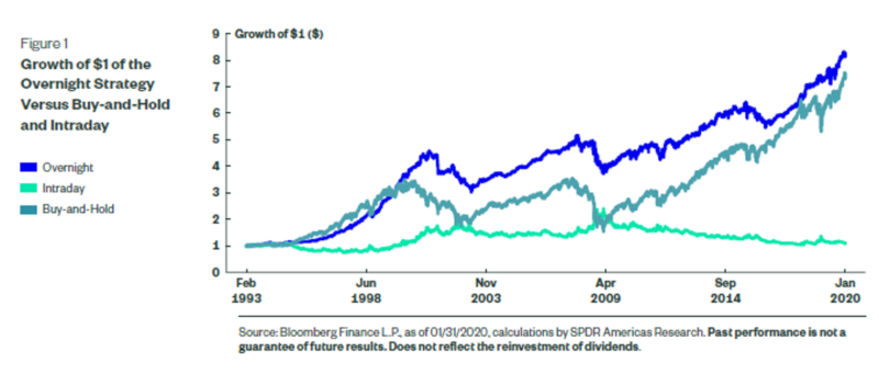
Figure 1 shows the growth of $1 from buying at the close and selling at the open (i.e., overnight) since 1993, without accounting for transaction costs, as compared with a buy-and-hold position of SPY and the intraday strategy (i.e., buy-at-the-open, sell-at-the-close) return. Cumulative price returns are 717%, 627%, and 12% for the overnight, buy-and-hold, and intraday strategies, respectively.
With cumulative returns like this, it’s no wonder that the idea of an overnight anomaly continues to receive attention in and out of academia. Articles published in The New York Times, Bloomberg, Business Insider, and other financial news(4) outlets have featured similar charts, only to stop the analysis there. And that’s the issue.
Random Walk or Time Dependent?
Even though we found the cumulative growth staggering versus the intraday performance, on only 53% of the 6,800 days analyzed was the daily return for the overnight higher than the intraday. The daily median performance overall was 0.05% for the overnight, versus -0.04% for the intraday, as the overnight strategy seemingly picks up pennies on a daily basis. To test whether or not the difference between the two return streams is significantly different than zero, we ran a paired sample t-test.
The test reveals that the difference between the two return streams is not meaningfully different than zero. The test results consist of a t-stat of 1.90 and a p-value of 0.06. This is below the t-stat threshold of significance of 1.96 and above our 5% level of significance. This test indicates that on a daily basis, a trading anomaly really doesn’t exist with any statistical significance.
But why the outperformance on a cumulative basis versus the intraday?
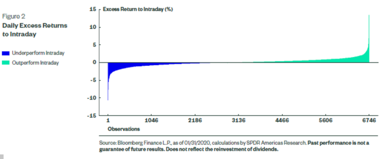
On average, our analysis shows that on a cumulative basis, the strategy can pick up pennies, and it sometimes even nabs a quarter, as there is a tailed nature to the return pattern. This point is reinforced by the statistical properties of the strategy. The overnight return stream has a kurtosis, a measure of the “tailedness,” of 17.68, which is significantly in excess of a normal distribution kurtosis level (3). Figure 2 depicts this tailed return distribution.
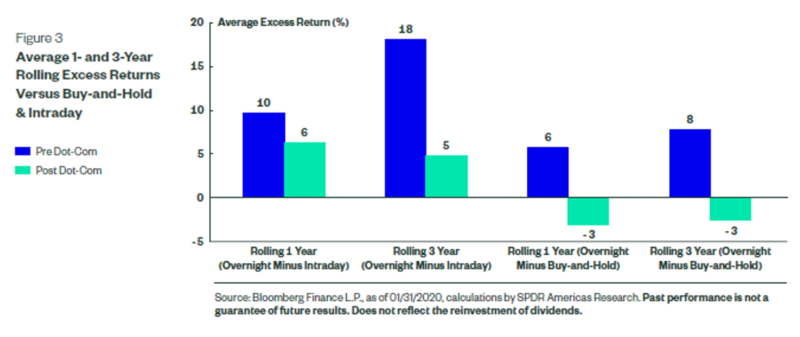
The tailed distribution doesn’t really answer the question of the strong cumulative returns, however. Digging deeper, though, reveals that most of the “excess returns” for intraday, as well as buy-and-hold, stem from the cumulative performance prior to the dot-com bubble(5). This is evident by looking at averages of rolling one- and three-year returns of the implemented strategy. As shown below, after the dot-com bubble, the overnight strategy’s average rolling one- and three-year excess returns over intraday and buy-and-hold were much lower than before the dot-com bubble.
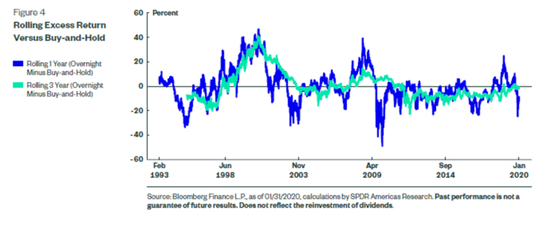
From a persistence perspective, relative to the buy-and-hold, the overnight strategy outperformed on 64% and 61% of the rolling one- and three-year periods, respectively, leading up to and until the end of the dot-com bubble. However, afterward, the trend is less persistent, with the exception of the great financial crisis, when idiosyncratic returns were common. In fact, post dot-com, the overnight strategy outperformed buy-and-hold in just 34% and 32% of periods on a rolling one- and three-year basis, respectively. Figure 4 illustrates this turn in the trend more acutely.
Random Walk in a March 2020 Bear Market
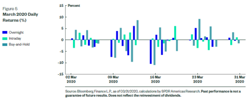
The random walk effect during periods of idiosyncratic market events can be further witnessed by examining the returns of the overnight, intraday, and buy-and-hold strategies in the month of March 2020, when the S&P 500 fell into a bear market for the first time since 2009.
As shown in Figure 5, the overnight strategy saw larger gains and larger losses than the intraday and buy-and-hold strategies on certain days as a result of the randomness of information/ news releases about the COVID-19 pandemic. This price action furthers the notion of the tailed distribution and the limited persistency of any market anomaly.
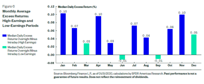
Earnings Seasonal Bias Provides Context
Seasonal analysis can provide context to the longer-term cumulative outperformance versus the intraday holding period. The next step in our analysis accounted for the impact of earnings periods, where the anomaly, per the theory, may have gotten an extra boost from the longstanding trend of positive price reactions from positive earnings surprises. Accounting for earnings season can provide insight as to whether this anomaly exists only during earnings season. As shown in Figure 6, using our methodology for quantifying high-earnings periods as discussed earlier, the excess returns of the overnight to intraday periods are greater in the high-earning months than in the low-earnings months[ref]High-earnings periods = January, February, April, May, July, August, October, November; Low-earnings periods = March, June, September, December.[ref].
The returns for each period were also chain-linked together to create one return stream, with the assumption that when it is not a high-earnings period, there are no returns, leaving the cumulative return stagnant. The process was also conducted for low-earnings periods. Therefore, as the compounding return is different, the two periods do not equal the total cumulative above. Higher returns could be achieved by rotating into cash-like vehicles (e.g., 3-month US Treasury Bills) and earn the associated income. But, to keep it simple, a zero return was assumed for those not-in-the-market periods.
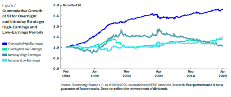
The cumulative return for the overnight strategy for high- and low-earnings periods is 177% and 46%, respectively. And the cumulative return spread of high earnings overnight (+177%) and high earnings intraday (7%) is much wider than low earnings overnight (+46%) and low earnings intraday (+36%), at 170% versus 10%, respectively. All of which provide support to the theory of harnessing earnings-related surprises. However, a lot of the return accumulation, as shown in Figure 7, is more visible prior to and during the dot-com bubble, and not so much after. This turn in the trend may be a result of a change in regulation, as Regulation FD (Reg FD) was implemented on October 23, 2000.
Reg FD eliminated much of the information advantage that analyst estimates had previously offered to institutional investors because of their privileged access to company management. As a result of the change in fundamental information dissemination, measured after Reg FD, the overnight high-earnings returns are less, as shown in Figure 8. Overnight high-earnings periods are still greater in both pre- and-post Reg FD. However, the spread between overnight high earnings and intraday high earnings, while still positive, is less post Reg FD.
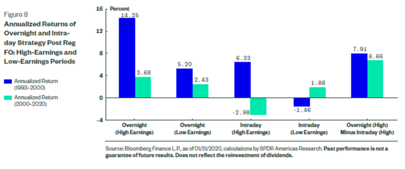
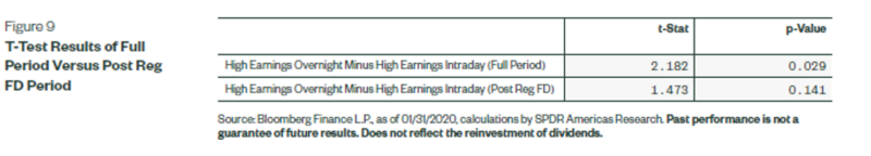
The positive return spread for the entire period, as it pertains to high earnings overnight versus high earnings intraday, is statistically significant different than zero, however — unlike when not controlling for just earnings periods. Running the same t-test as above, the t-stat is 2.1 with a p-value of 0.03 for high earnings overnight minus high earnings intraday for the entire period. However, the return spread is not significantly different than zero when only considering post Reg FD.
That Was Then, This Is Now
The summary for both t-stat tests below confirms that the anomaly between the trading strategies was more persistent earlier in history than it is now. Despite these statistical findings, the notion of this market timing strategy’s strong cumulative returns continues to get attention. However, implementing this strategy requires persistent capital and exposure — all of which come at a cost, further reducing the viability of the overnight strategy.
The Trading Costs of Being up at Night
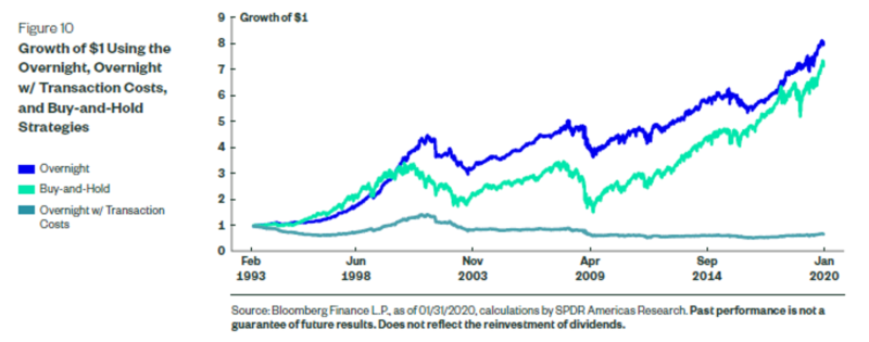
There is a cost to implementing any strategy, and especially a strategy such as this, which relies heavily on trading. Figure 10 illustrates the impact of both commissions and the bid-ask spread. For an overnight strategy that does incur trading costs, the cumulative return would be -32%, versus the no-transaction cost strategy of 717%. The 749% difference underscores the sizable impact trading costs can have. The aspect of outperforming the market completely disappears and refutes the notion that buying at night and selling in the morning offers any premia.
Applying this to only high-earnings seasons has the same result; the cumulative return drops from 177%, as mentioned earlier, to 12% once transaction costs are included. Buy-and-hold returns during high-earnings periods are 215%, leading to sizable negative excess returns for the overnight strategy.
The overnight market strategy appears to be effective prior to the dot-com bubble and Reg FD during high-earnings periods, consistent with the theory of capturing fundamental news surprises. However, it appears to lose much of its effectiveness when factoring in all transaction costs — meaning it’s unlikely to work in the real world or result in any performance premia.
This analysis illustrates the extreme impact that trading strategy and transaction costs can have on overall performance:
- Strategy evaluation: What are the explicit trading costs of the asset/fund/exposure;
- Implementation: What is the turnover of the asset mix and;
- Execution when rebalancing: How frequently will the strategy be rebalanced and what are the implicit (i.e., market-slippage costs) associated with it
All told, disproving a popular timing strategy underscores the need to consider all parts of the total cost of ownership equation in the due diligence process. As the time horizon extends and the number of times an asset is traded increases, those costs will eat away at a strategy’s returns — anomalous or otherwise.
References[+]
| ↑1 | Source: FactSet, as of 01/31/2020. |
|---|---|
| ↑2 | Source: FactSet, as of 01/31/2020. Companies over the past five years have, on average, witnessed a 1.0% price increase two days before the earnings release through two days after the earnings. |
| ↑3 | “Buyback Blackout Periods Do Not Negatively Impact Performance”, Bartolini, Kaplanian 2019. |
| ↑4 | A Winning Trade: Buy S&P 500 ETF at Market Open, Sell at Close, Bloomberg 4/6/2020, This wacky daily trading strategy posted a 13% return in this rough year, CNBC.com December 31, 2018 The Stock Market Works by Day, but It Loves the Night, New York Times February 2018; Buy the close, sell the open, Business Insider March 2016 . |
| ↑5 | End of the dot-com bubble is defined as 12/31/2002. |
About the Author: Matthew Bartolini
—
Important Disclosures
For informational and educational purposes only and should not be construed as specific investment, accounting, legal, or tax advice. Certain information is deemed to be reliable, but its accuracy and completeness cannot be guaranteed. Third party information may become outdated or otherwise superseded without notice. Neither the Securities and Exchange Commission (SEC) nor any other federal or state agency has approved, determined the accuracy, or confirmed the adequacy of this article.
The views and opinions expressed herein are those of the author and do not necessarily reflect the views of Alpha Architect, its affiliates or its employees. Our full disclosures are available here. Definitions of common statistics used in our analysis are available here (towards the bottom).
Join thousands of other readers and subscribe to our blog.