We have all heard the mantra, “You can’t time the market!” But in reality, investors attempt to do just that every day as part of their tactical asset allocation strategies, which are less extreme variants of the classic trend-following “risk-on/risk-off” approach, which many associate with market timing.(1)
Moreover, numerous studies have shown that institutional investors routinely outperform individual investors over intermediate time horizons(2)(3) (4)(5). These results are deep and robust—holding across different metrics, different markets, and different time periods—and not terribly surprising given the inherent and persistent structural advantages institutions have over individuals (such as better information networks, deeper human capital resources, and more advanced technological infrastructure).
In light of these studies, we hypothesize that what institutions are doing in the financial markets may provide predictive insights.
In that context, in a recent SSRN paper (“Want Smart Beta? Follow the Smart Money: Market and Factor Timing Using Relative Sentiment”), we present a real-time, cross-asset, positions-based relative sentiment indicator to quantify exactly which side of the trade institutions are on.
Derived from the Commitments of Traders (COT) report, the indicator measures—in a novel way—the aggregate positioning in equities of institutional investors relative to individual investors. For simplicity, we refer to the indicator as the Smart Money Indicator (SMI), as institutional investors are often thought of as the “smart money.”(6)
The main findings of the paper are as follows:
- The SMI and market timing: Institutional investors have demonstrated highly significant market timing ability over the 25-year history of the weekly COT report. This significance is both economic and statistical; is evident in both halves of the dataset; passes extremely stringent data snooping tests; and is exceptionally robust to different parameter combinations, lags in the data, and methods of computing the indicator.
- The SMI and momentum: Regardless of the state of the market’s time-series momentum (i.e., “trend”), returns are significantly higher (lower) when the SMI is positive (negative). This effect is especially pronounced when the market has negative time-series momentum. In such cases, annualized market returns are (on average) +30% when the SMI is positive, and -20% when the SMI is negative—a spread of 50 percentage points. In other words, the SMI appears to be adept at identifying when (and when not) to take equity market exposure during periods of negative time-series momentum.
- The SMI and smart beta factors: While conventional wisdom tends to hold that smart beta equity factors are difficult, if not impossible to time,(7)(8) the polarity of the SMI appears to largely determine the general return outcomes for several fundamentally-based long/short equity factors. In addition, both the statistical and economic significance of the SMI-based factor timing become quite strong when we further condition the timing on the state of the factors’ time-series momentum.
- The SMI versus value and momentum: We develop a walk-forward tactical asset allocation (TAA) strategy using the SMI and compare it to several value- and/or momentum-based alternatives. Here we see that over the last 20 years, the SMI has been more efficient at identifying higher-yielding equity market opportunities than either value or momentum (or a combination of the two). That is, the SMI-based strategy has produced higher returns (both absolute and risk-adjusted) with generally lower drawdowns, while spending considerably less time invested in equities than its value or momentum counterparts.
- Cross-hedging pressure is the key: de Roon et al. (9) show that futures risk premia depend not only on investors’ positions in the futures contract under consideration, but also on their positions in closely-related assets (so-called “cross-hedging pressure”). The key innovation of the SMI is that it looks not only at investors’ positions in equities, but also at their positions in long-duration bonds and along the yield curve. Tests show that all three components are vital to the predictive power of the SMI.
Data and Testing Details
We use data from the weekly COT report to compute the SMI. The data spans the time period October 6th, 1992 to December 29th, 2017 (and encompasses 1150 weekly data points). To account for the evolution of the COT report’s accessibility during a portion of the time period under consideration, we incorporate a one-week lag of the COT data for our primary results.
To administer the factor timing tests (of which market timing is a special case), we use factor returns obtained from Professor Kenneth R. French’s data library and from AQR’s data library.
Smart Money Indicator
The SMI is the additive combination of three “institutional-versus-individual” relative sentiment (IIRS) components.
These components include the following:
- Equities IIRS: A measure of relative sentiment in the large S&P 500 futures contract
- Long-Duration IIRS: A measure of relative sentiment in the 30-Year U.S. Treasury Bond
- Yield-Curve IIRS: A measure of the difference in relative sentiment between the 10-Year U.S. Treasury Note and the 30-Year U.S. Treasury Bond.
The first component is a direct measure of IIRS in equities.
The second component functions as an indirect—and inverse—measure of IIRS in equities. Given the general inverse relationship between equities and long-duration bonds, if institutions are relatively bearish long-duration, that might imply they are relatively bullish equities (and vice versa). This conjecture has empirical support, as de Roon et al. find strong cross-hedging pressure between the S&P 500 and the U.S. Treasury Bond.
Similarly, the third component also functions as an indirect measure of IIRS in equities. The idea here is that if institutions are relatively long shorter-duration assets (i.e., relatively longer the 10-year Note than the 30-year Bond), that might imply they are expecting long-duration assets to fare relatively poorly. And, given the general inverse relationship between long-duration and equities, that might correspondingly imply institutions are expecting equities to perform relatively well.
We use composite z-scores to quantify the three IIRS components. We then add those components together, subtract off the cumulative median value to arrive at the SMI, and test whether its sign is predictive. (The paper provides details of the computation.)
By its construction, the SMI ends up being a function of two parameters, which we label N and M. N is the lookback length (in weeks) of the underlying z-scores, and M is a lookback length (in weeks) over which we compute the trailing maximum or minimum value of each IIRS component. (These extrema computations essentially smooth out the directional signals of the SMI and reduce whipsaws.)
It should be emphasized that the SMI is purely a relative indicator. Thus, institutions could be net short (long) equities in the aggregate, yet still be relatively longer (shorter) than they typically are, causing the SMI to be positive (negative).
Moreover, given that institutions expend considerable resources attempting to ascertain the ongoing state of corporate and economic fundamentals, how they hedge their equity and bond portfolios in the futures markets is essentially their consensus opinion on the state of those fundamentals. In that sense, the SMI may perhaps best be thought of as an implied fundamental indicator.
Statistical Tests for Factor Timing
To test the robustness of the SMI, we consider 6 different values for N (namely, 39, 52, 65, 78, 91, and 104 weeks, corresponding to 3, 4, 5, 6, 7, and 8 quarters, respectively) and 13 different values for M, ranging from 1 to 13 weeks. Further, we use the same M value for each IIRS component. (That is, we make no effort to find either an optimal N value or an optimal combination of M values.)
With 6 N values and 13 M values, there are 78 pairwise SMI parameter combinations, and thus 78 individual SMI time-series. Given our focus on the SMI’s sign, each SMI time-series generates two sets of conditional returns—the set of weekly factor returns when the prior-week SMI is positive and the set of weekly factor returns when the prior-week SMI is negative. (We denote these sets of returns for factor F as R(F, SMI+)t and R(F, SMI—)t, respectively.)
Moreover, each SMI time-series also generates two “long-or-flat” factor timing strategies. The first goes long factor F when the prior-week SMI is positive and is flat otherwise (see here for an example of this approach with traditional trend following). The second goes long factor F when the prior-week SMI is negative and is flat otherwise. We denote these strategy returns by S(F, SMI+)t and S(F, SMI—)t, respectively.
These conditional returns and long-or-flat factor timing returns serve as inputs to eight different factor timing tests. The appendix of the paper provides the implementation details of these tests (e.g., how we incorporate different asset pricing models into the analysis, how we handle heteroskedasticity, autocorrelation, and outliers, and so on).
Because we use one particular test to account for autocorrelation in three distinct ways, these eight tests produce 11 separate p-values of factor timing significance for each SMI parameter combination. We compute the median of those 11 p-values at each parameter combination to arrive at a 13 x 6 matrix of median p-values. This matrix conveys two things: 1) How broadly significant any individual SMI parameter combination is, and 2) how robust the SMI is across all parameter combinations.(10)
We further compute the differences in annualized returns and volatilities between the two sets of conditional returns described above (i.e., R(F, SMI+)t and R(F, SMI—)t) at each SMI parameter combination (resulting in two 13 x 6 matrices). The differences in annualized returns provide a measure of the SMI’s economic significance, while the differences in annualized volatilities reveal whether the SMI state with higher returns also has higher volatility (as modern portfolio theory would predict).
Lastly, we employ a test that controls for data snooping—the (bootstrap-sampling-based) Multiple Hypothesis Testing algorithm of Romano and Wolf(11). This test takes as inputs an integer, k, representing an allowable number of false positives and a probability, α, such that P{Number of false positives > k} ≤ α.
We set k = 1 and consider α values of 0.10, 0.05, 0.01, and 0.001. Romano et al. (12) state that typical α values are 0.10 and 0.05. However, de Prado and Lewis (13) show that values of α less than 0.15 tend to be overly restrictive (i.e., generate too many false negatives). In this context, the values of α used in the paper appear to be sufficiently, if not excessively, conservative.
The paper presents two sets of results from the MHT algorithm. One set corresponds to the raw, unadjusted bootstrap samples. The other set corresponds to constraining the potential oversampling of time-localized outliers—both positive and negative—in the bootstrap samples.
In order to gauge the broad performance of the SMI across all the aforementioned metrics, we present tables that summarize the number of SMI parameter combinations whose median p-values exceed certain significance levels, the number with differences in annualized returns and volatilities beyond certain thresholds, and the number deemed significant by the MHT algorithm (as a function of k and α, with and without adjustments for outliers).
Smart Money Market Timing
To give one a visual sense of the SMI’s ability to time the “market factor” (i.e., the market minus the risk-free rate, which we denote by MRF), we first plot the cumulative compounded returns of S(MRF, SMI+)t versus S(MRF, SMI—)t. Here, we set N = 78 and M = 5 (this parameter combination was selected because it has the median p-value from among a large contingent of the more statistically significant parameter combinations).
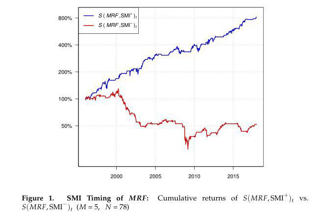
Over the 22-year period from December 22, 1995 until December 29, 2017, $1 invested in the positive-SMI strategy would have grown to $8.20, while $1 invested in the negative-SMI strategy would have fallen to 52 cents (i.e., one would have lost 48%). On an annualized basis, the difference in those two streams of returns is 27.2 percentage points. At the end of the period, the positive-SMI portfolio was worth roughly 16 times the negative-SMI portfolio. As a frame of reference, it took over 62 years (1926-1988) for a portfolio representing the top quintile of value stocks to be worth 16 times a portfolio representing the top quintile of growth stocks.
While impressive, the performance of this particular SMI parameter combination is not an isolated event. Nor is the general performance of the SMI fragilely dependent on its precise method of construction. To demonstrate this robustness, we consider 15 other computational variants of the SMI. These variants differ mainly based on the underlying COT data (futures-and-options vs. futures-only), the lag of the COT data (0-, 1-, or 2-week lags), and the time period covered (entire period, first half, or second half).
However, we also consider other variants, such as incorporating the S&P 500 E-mini contract into the computation (Case 5) or alternately subtracting off the rolling 3-year median (Case 6) or the cumulative 40th percentile (Case 7) rather than the cumulative median in the SMI’s construction. Further, we analyze each of the SMI’s IIRS components (i.e., equities, long-duration, and yield-curve) separately and in groups of two (Cases 8-13).
The following table lists the specifics of each case:
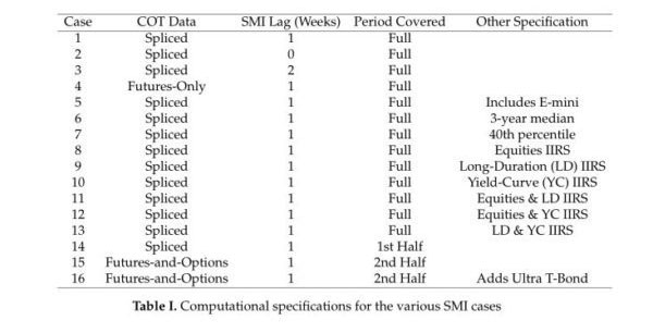
Note: “Spliced” data indicates that we spliced futures-only data from 1992-1995 with futures-and-options data from 1995 onward (when it became available).
The following table presents a statistical summary for each of these computational cases:
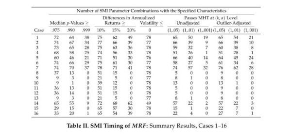
For the baseline case, Case 1 (which analyzes the full time period, uses spliced COT data, and incorporates a one-week COT lag), 72 of 78 SMI parameter combinations have median p-values greater than 0.975 (i.e., significant at the 0.025 level), 64 have median p-values greater than 0.99 and 38 have median p-values greater than 0.999. At the extremes, we observe t– and z-stats as high as 6 for certain SMI parameter combinations and certain factor timing tests.
In terms of economic significance, 49 parameter combinations have differences in annualized returns greater than 20 percentage points (which also happens to be the average difference across all 78 parameter combinations for Case 1). Further, the differences in annualized volatilities are negative for all SMI parameter combinations–indicating that the higher returns when the SMI is positive come with lower volatility.
Lastly, when controlling for data snooping (using the raw, unadjusted bootstrap data), 65 parameter combinations are deemed significant at the α = 0.05 level, 50 are deemed significant at the α = 0.01 level, and 19 are deemed significant at the unusually stringent α = 0.001 level. These latter results all but verify the market timing performance of the SMI is likely not the product of data mining.
Cases 2-7 also analyze the full dataset—altering either the underlying COT data, the lag of the COT data, or the method of constructing the SMI. Each of these cases exhibits roughly similar levels of statistical significance as Case 1.
This robustness with respect to its precise construction method, dataset, or lag period suggests the SMI’s polarity is somehow able to capture the inherent forecasting advantages institutions have over individuals, along with the time horizons over which build-ups in sentiment unwind (the average holding period of the more significant SMI parameter combinations is approximately 16 weeks).
Cases 8-13 analyze the individual components of the SMI separately and in groups of two across the entire dataset. As is evident from the table, the statistical and economic significance of these cases pale in comparison to that of Cases 1-7. The obvious inference, then, is that the predictive power of the SMI must largely stem from combining the hedging pressure of equities with the cross-hedging pressures from long-duration bonds and from along the yield curve.
Cases 14 and 15 analyze the first and second halves of the dataset, respectively. Thus, they encompass half as many data points and therefore have less power to identify extreme statistical significance. Nonetheless, both cases have a substantial number of parameter combinations indicating high significance. For the first half of the data set (Case 14), 55 parameter combinations have median p-values greater than 0.99, 62 have differences in annualized returns greater than 20 percentage points, and 57 are deemed significant by the outlier-adjusted MHT algorithm at the α = 0.05 level. For the second half of the dataset (Case 15), the corresponding numbers are 15, 30, and 22.
The relatively fewer number of highly significant parameter combinations in Case 15 was a function of two phenomena. The first is that the second half of the dataset covers the Great Recession and there was a cluster of “slower-moving” SMI parameter combinations (i.e., ones with higher N and M values) that were vulnerable to incorrect forecasts during that time period.
The second is the 2010 launch of Ultra Treasury Bond futures. These contracts have an even longer duration than regular Treasury Bond futures. Consequently, these Ultra Treasury Bond futures absorbed some of the long-duration positions that otherwise would have been expressed in regular Treasury Bond futures. When we factor these Ultra Treasury Bond futures into the construction of the SMI (Case 16), noticeably more parameter combinations exhibit high significance—which once again underscores the importance of accounting for relevant cross-hedging pressures in the construction of the SMI.
Smart Money Momentum Timing
In light of the SMI’s performance timing the broad market, it’s natural to ask whether the SMI adds any incremental information beyond that provided by the market’s time-series momentum (TSM). What we find instead, however, is precisely the opposite: In the presence of the SMI, TSM adds no statistically significant information in predicting U.S. equity returns.
This is most clearly illustrated by the SMI’s ability to “time” negative TSM. That is, its ability to identify when (and when not) to take equity exposure when the market’s TSM is negative.
We begin by plotting the cumulative compounded returns generated by the following two long-or-flat timing strategies:
- Strategy 1: Be long MRF when the prior-week SMI is positive and the prior-week TSM is negative, otherwise be flat (denoted S(MRF, SMI+, TSM—)t)
- Strategy 2: Be long MRF when the prior-week SMI is negative and the prior-week TSM is negative, otherwise be flat (denoted S(MRF, SMI—, TSM—)t)
As before, we set N = 78 and M = 5, and the SMI corresponds to Case 1 above (i.e., spliced COT data, one-week lag).
(Note: We use two different momentum indicators to identify the state of TSM. The first is an intermediate-term total return and the second is a longer-term moving average. To check robustness, we consider three different day-lengths for the first indicator (namely, 63, 84, and 105 days, corresponding to 3, 4, and 5 months, respectively) and three different day-lengths for the second indicator (i.e., 150, 200, and 250 days), leading to 9 pairwise parameter combinations to quantify TSM. The cumulative strategy returns in the following plot are composites, averaged across all 9 TSM parameter combinations.)
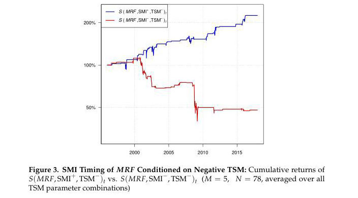
One dollar invested in Strategy 1 would have grown to $2.25, while $1 invested in Strategy 2 would have fallen to 48 cents, a loss of 52%. This latter result highlights the potential danger of being long the market when both TSM and the SMI are negative.
The following table summarizes the timing performance of the 78 SMI parameter combinations conditioned on negative TSM—for each TSM parameter combination. (Note: We denote the different TSM parameter combinations by “ij-,” where i represents the i-th element of the intermediate-term total return parameter vector, j represents the j-th element of the longer-term moving average parameter vector, and the “-“ sign indicates conditioning on negative TSM. Thus, “22-“ would indicate that TSM was identified using the second element of the day-length parameter vector for both the intermediate-term total return and longer-term moving average, which in this case would be an 84-day total return and a 200-day moving average.)
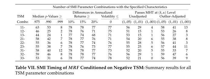
From the above table, we can see that for each TSM parameter combination, upwards of several dozen SMI parameter combinations have median p-values greater than 0.99. Likewise, several dozen SMI parameter combinations are deemed significant by the outlier-adjusted MHT at the α = 0.01 level (which is an especially extreme threshold in this case because periods of negative TSM represent only 24% of the entire sample of 1150 weekly data points).
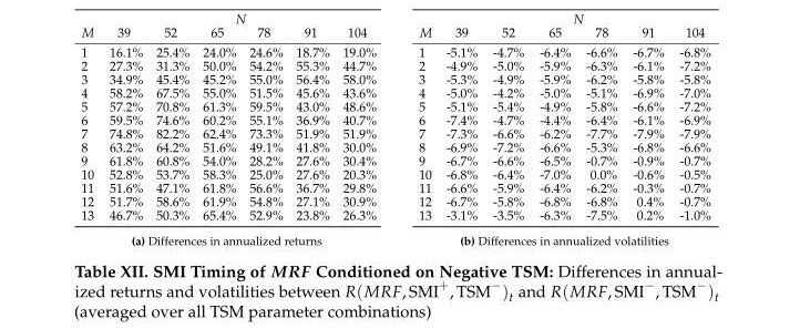
But perhaps the most interesting result of the paper is the economic significance of the SMI’s ability to time negative momentum. The following tables show the average difference–averaged across all 9 TSM parameter combinations–in annualized returns and volatilities for each SMI parameter combination when TSM is negative.
The results are hypothetical results and are NOT an indicator of future results and do NOT represent returns that any investor actually attained. Indexes are unmanaged and do not reflect management or trading fees, and one cannot invest directly in an index.
Taking the average across all SMI parameter combinations in the table on the left, we get an average return spread of 50 percentage points. Breaking this down: When TSM is negative, but the SMI is positive, the market (on average) returns 30% annualized. When TSM and the SMI are both negative, the market returns -20% annualized. Thus, the SMI appears adept at identifying when (and when not) to take equity exposure during periods of negative time-series momentum.
As one of the weaknesses of momentum as a TAA indicator is that it tends to maintain reduced (or zero) allocations to equities well after the market has bottomed, momentum-based investors are perpetually susceptible to missing out on the often-substantive returns that tend to occur right after significant market troughs—as they wait for momentum indicators to turn positive. The foregoing results suggest that by monitoring the SMI, momentum-based investors might be able to participate more fully in those post-trough rebounds.
Smart Money Factor Timing
Next, we examine the SMI’s ability to time the following smart beta factors:
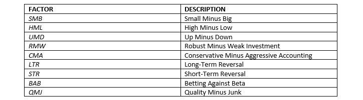
We observe three types of factors:
- Group 1: Those that do better when the SMI is positive (SMB, STR)
- Group 2: Those that do better when the SMI is negative (HML, RMW, CMA, LTR, BAB, QMJ)
- Group 3: Those that exhibit no evidence of SMI timability (UMD)
The results for Group 1 are only weakly significant, thus our focus here will be on Group 2 factors.
To get a visual sense of the SMI’s ability to time Group 2 factors, we plot the cumulative compounded timing returns for a selection of these factors (namely, HML, RMW, BAB, and QMJ). For each figure below, the SMI parameter combination corresponds to the one with the median p-value from among a selection of the more significant ones (for the factor under consideration).
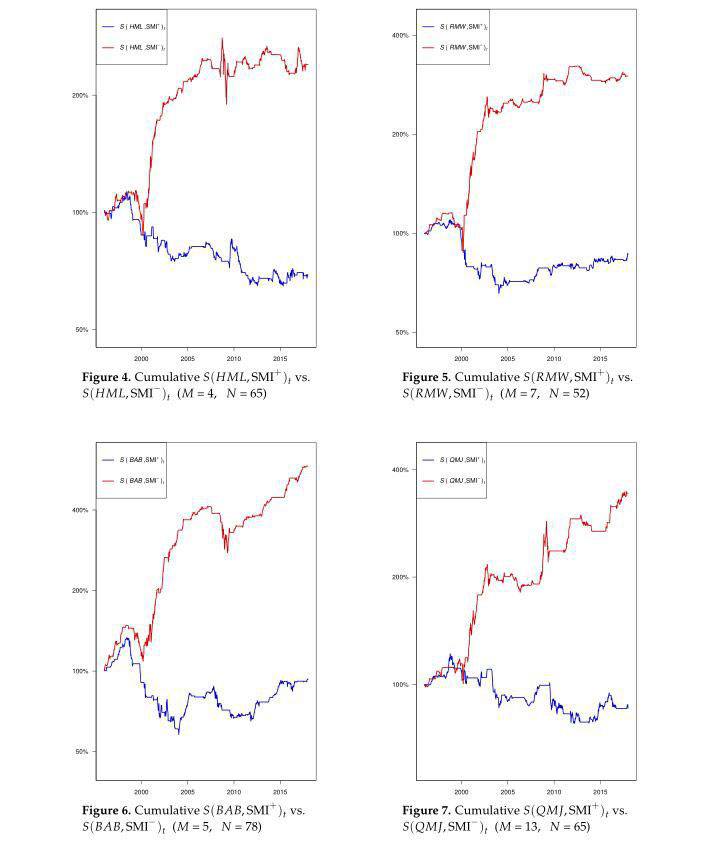
From the figures, we see that Group 2 factors tend to drift sideways or higher when the prior-week SMI is negative (red) and sideways or lower when the prior-week SMI is positive (blue).
The following table presents the summary results for the Group 2 factors. Factor symbols followed by a “+” sign indicate the factor timing was further conditioned on the factor having positive TSM.
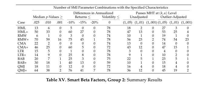
Based on the data snooping results, the SMI, by itself, has moderately strong timing ability for Group 2 factors, and strong-to-exceptionally-strong timing ability when the factors are in a state of positive TSM. For example, when timing HML unconditionally, 27 parameter combinations pass the outlier-adjusted MHT algorithm at the α = 0.05 level. When we condition on HML having positive TSM, 53 parameter combinations register as significant at that same level, while 25 are now deemed significant at the α = 0.01 level (and 4 at the α = 0.001 level). RMW really stands out in this regard–when RMW has positive TSM, virtually all of its parameter combinations are significant at the (outlier-adjusted) α = 0.05 level, and 23 parameter combinations are deemed significant at the α = 0.001 level.
Group 2’s results appear to agree with observed market behavior. As Group 2 factors are based on fundamentals or proxies for fundamentals, their short portfolios tend to consist of expensive, low-quality “glamour” stocks. “Risk-on” (i.e., SMI-positive) markets tend to reward these glamour stocks, which causes long/short factor performance to suffer. In contrast, “risk-off” (i.e., SMI-negative) markets tend to penalize glamour stocks and reward quality, which leads to improved long/short factor performance.
Smart Money Tactical Asset Allocation
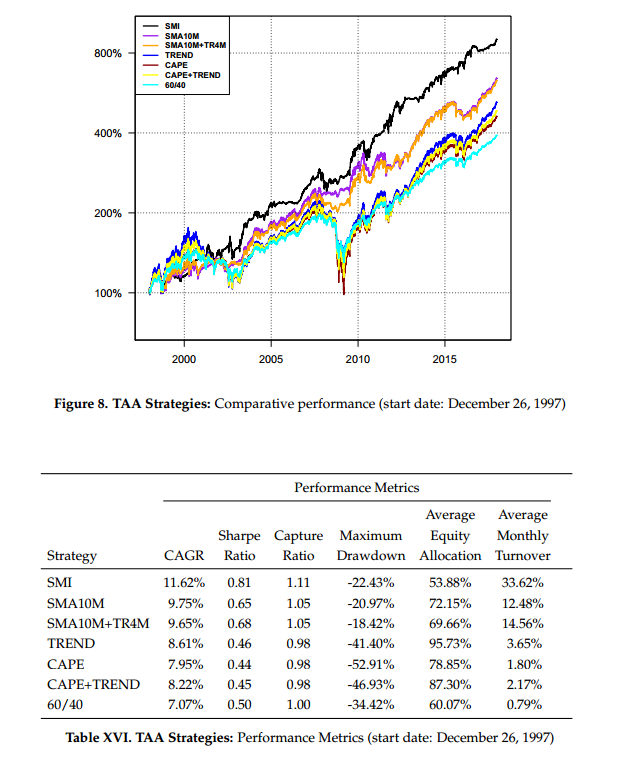
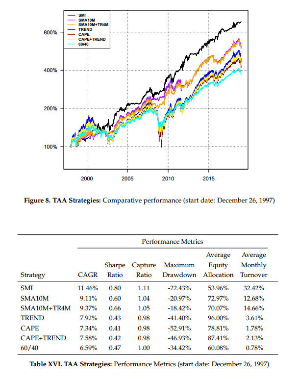
In the paper, we develop a walk-forward TAA strategy based on the SMI (with estimations of transaction costs, slippage, and management fees included) and compare it to the following alternative strategies:
- 60/40: A passive 60/40 consisting of U.S. equities and bonds, rebalanced quarterly
- SMA10M: The 10-month moving average strategy (14), which is 100% in equities when the market is above its 10-month moving average, and 100% in bonds otherwise
- SMA10M + TR4M: A variant of the 10-month moving average strategy that looks at both the 10-month moving average and the 4-month total return (15). If both are positive, the strategy is 100% equities. If only one is positive, the strategy is 50% equities, 50% bonds. And if both are negative, the strategy is 100% bonds.
- CAPE + TREND: This is the value-and-momentum strategy presented in Asness et al. (16), which combines the (inverse of the) Cyclically-Adjusted Price-to-Earnings (CAPE) ratio with a 12-month trend indicator. (Note: the equity allocations in this strategy range from 50%-150%, rather than 0%-100% as with the other strategies). We also present results for CAPE and TREND standalone.
The time period of the backtest is 1997-2017. For each strategy, we average the results from three different execution variants to better simulate real-world portfolio management conditions. For example, for the SMI strategy, one variant trades on Thursday, one trades on Friday, and one trades on the following Monday. For the month-end strategies, one variant trades on the second-to-last day of the month, one trades on the last day of the month, and one trades on the first day of the following month.
The trading vehicles we use are the broad U.S. equity market (represented by returns from Professor Ken French’s data library) and an aggregate bond index (represented by the Bloomberg Barclays Aggregate Bond Total Return Index).
We assume four basis points of detrimental slippage relative to the closing prices on the day of execution, commissions of $4.95 per trade, and a 15 basis-point management fee (with the exception of the 60/40 strategy).
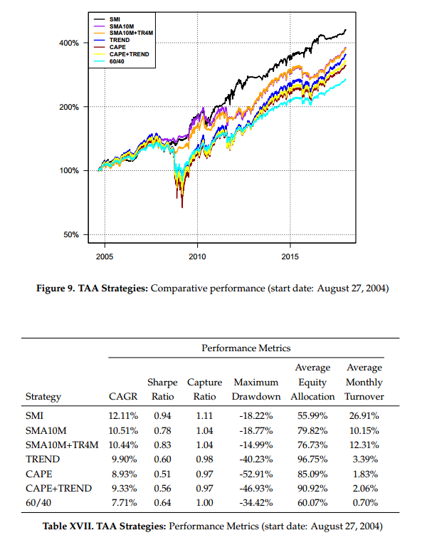
Below we show results across the entire backtest, as well as starting 1/3rd and 2/3rds of the way through the time period.
And here are the results when we start 1/3 of the way in the sample:
And here are the results when we start 2/3 of the way in the sample:
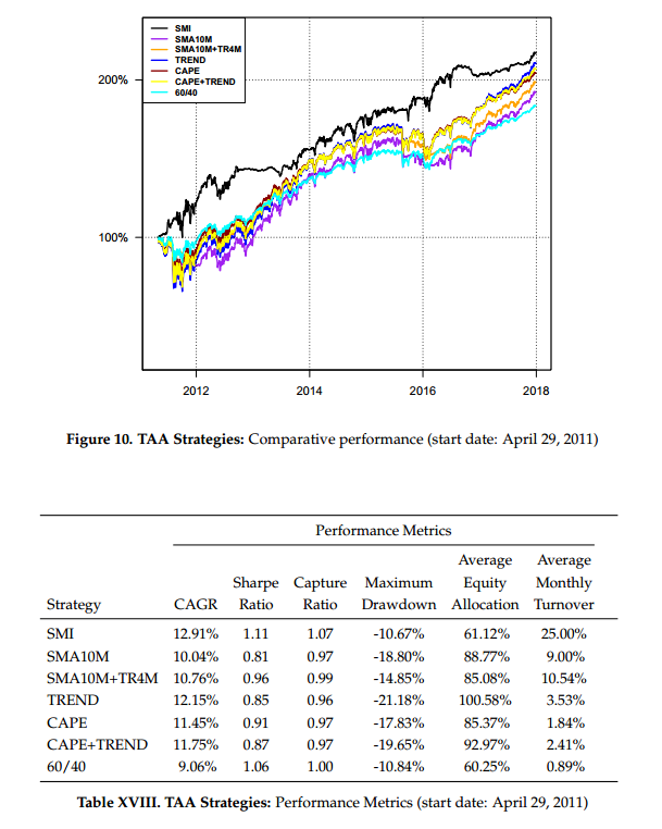
From the figures and tables, we see the SMI-based strategy, over all time periods, generated higher returns with higher Sharpe ratios, higher capture ratios, and generally lower drawdowns, while spending much less time invested in equities than its active counterparts. This suggests the SMI may be both more powerful and more efficient at identifying higher-yielding equity market opportunities than either value or momentum (or their combination).
Notably, over the 2011-2017 time period, a period during which equity markets rose strongly–and it was generally detrimental not to be fully invested in equities–the SMI strategy outperformed its closest competitor, TREND, by 75 basis points per annum while having a time-averaged equity exposure of only 61% compared to 101% for TREND.
The efficiency of the SMI strategy does come at the cost of higher average monthly turnover, however. This turnover can be mitigated somewhat by rebalancing the SMI strategy at month-end (similar to the other strategies) with little change in performance.
Updated TAA Results Through 2018
Given that we now have a full year of out-of-sample data, we present the full-period results extended through 2018:
In 2018, the SMI strategy benefited from its rotation out of equities into bonds in early August, about six weeks before the eventual 2018 high.
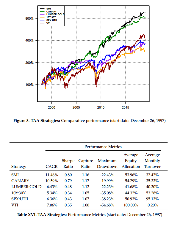
Comparison with Cross-Asset Strategies
While not in the paper, we recently ran comparisons between the SMI strategy and various cross-asset TAA strategies found in the literature. The cross-asset strategies we examine include:
- CANARY: The CANARY strategy (17)(which was recently written up in this space) looks at the month-end “fast” weighted averages of EEM and BND to determine whether to be in equities or bonds for the following month. If both fast moving averages are positive, the strategy is long equities. Otherwise, the strategy is long bonds.
- LUMBER:GOLD: The LUMBER:GOLD strategy (18) looks at the lumber-to-gold ratio. If the lumber is outperforming gold over the trailing 13 weeks, the strategy is long equities for the following week. Otherwise, it is long bonds. (For lumber and gold performance, we used roll-adjusted continuous front-month futures.)
- 10Y:30Y: The 10Y:30Y strategy (19) looks at the trailing month’s return of the 10-year bond relative to the 30-year bond. If the 10-year outperforms the 30-year, the strategy is long equities the following month. Otherwise, the strategy is long bonds. (We use roll-adjusted continuous futures for the 10-year and 30-year bond returns.)
- SPX:UTIL: The SPX:UTIL strategy (20) compares the four-week return of the S&P 500 to the four-week return of the utilities sector. If the S&P 500 has outperformed over that period, the strategy is long the S&P 500 over the next week. Otherwise, the strategy is long the utilities sector. (In order to provide an apples-to-apples comparison across strategies, however, whenever the strategy wants to be long utilities, we invest in an aggregate bond index instead.) Here is a review of this paper by Alpha Architect.
- VTI: As a benchmark, we consider a buy-and-hold strategy on the Vanguard Total Market Index.
As before, we consider three different execution variants. Moreover, we use the same assumptions with regards to trading vehicles, transaction costs, slippage, and fees. Below we present the backtest results for the entire time period (1997-2018) and for the last third of the time period (2011-2018). From the chart and table, we see that over the full period the SMI and CANARY strategies were quite similar in their performance and risk characteristics–both solidly outpacing the other strategies as well as the broad market (VTI).
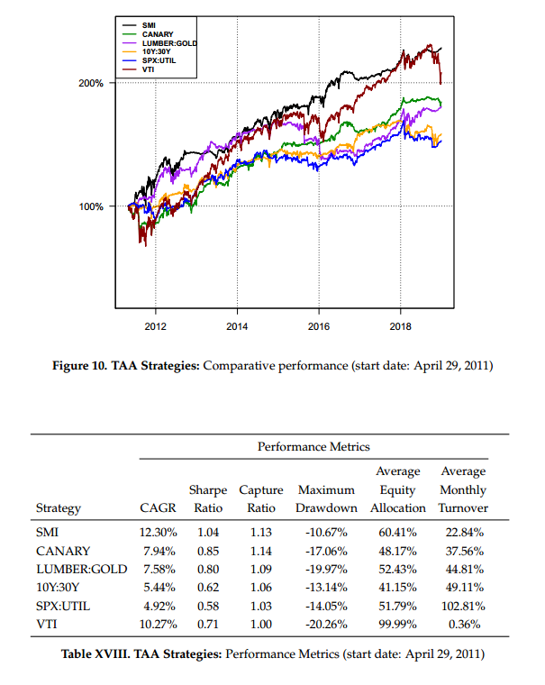
Over the last third of the time period (2011-2018), however, the SMI strategy appears to have begun separating itself from the pack:
Additional Results
The following results are also not in the paper but were generated based on suggestions and inquiries from Wes.
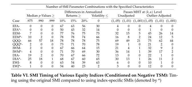
We first look at the SMI’s ability to time equity index ETFs other than the S&P 500 (namely, EFA, EEM, QQQ, IWM, DIA, and EWJ—the underlying indices of which all have their own COT data). The following table displays the summary results using both the original SMI and index-specific SMIs found by substituting the indices’ own COT data for the equities IIRS component of the SMI. (For example, when timing QQQ, substituting the Nasdaq 100 COT data in place of the S&P 500 COT data, and so on.) We denote the index-specific results with an asterisk after the ETF symbol. For each index, the two sets of results are computed over the same time period (but the time periods differ between indices based on the historical availability of the index-specific COT data).
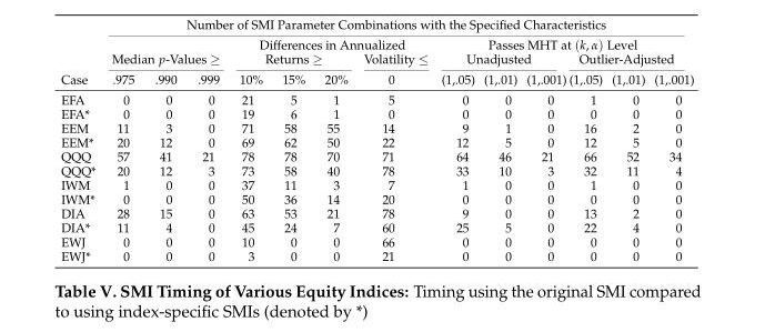
For some indices, the original SMI has more predictive power (e.g., QQQ), while for others, their own COT data adds value (EEM, DIA). Both EWJ and EFA (whose largest allocation is to Japanese equities) exhibit little or no statistical significance, but some signs of economic significance (i.e., differences in annualized returns). IWM also shows low statistical significance but fairly strong economic significance. (Note: The COT data for EFA, EEM, and IWM have relatively short histories.)
We next examine the same equity index ETFs when they have negative TSM to see whether the original SMI or the index-specific variants can time those indices during such periods. The results are presented in the following table (as before, we denote the index-specific results with an asterisk):
Notably, both the original SMI and the index-specific SMIs all show strong economic significance when timing the indices during periods of negative TSM (i.e., several dozen parameter combinations with differences in annualized returns greater than 20 percentage points). The data snooping significance is also much higher across the board and now even registers for EFA, EWJ, and IWM. It thus appears the SMI may be capable of timing negative momentum for indices beyond the S&P 500 (not surprising given the correlations among equity indices).
Next, we look at the cross-sectional behavior of the SMI. Here we compute SMIs for each of the six indices listed above plus the S&P 500—substituting in the index-specific COT data for the equities IIRS component of the SMI. We then rank the SMIs each week and record the subsequent weekly returns corresponding to each of the different positions within the ranking hierarchy. We concatenate the respective returns each week to form time-series corresponding to each of those ranks. We do this for N values of 52, 65, and 78 and for M values of 5 through 9 (roughly the sweet spot of the SMI’s predictive power) and average the resulting time-series of returns at each ranking position. We take those time-series of average returns and compound them to arrive at a total return for each ranking position. Below is a plot of these total returns corresponding to the different ranks along the cross-section, from lowest to highest.
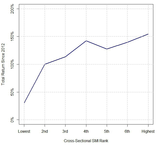
The returns are roughly a monotonically increasing function of the rank. Further, looking at the frequency at which the indices appeared at the top or bottom of the rankings, we see that the two indices with the highest returns since 2012 (the date when all indices have COT data available), SPY and QQQ, appeared at the top of the rankings with the highest frequency. Likewise, the two indices with the lowest returns over that time span, EFA and EEM, appeared at the bottom of the rankings with the highest frequency. These preliminary results suggest index-specific variants of the SMI might be helpful in predicting relative equity returns.
2018 Out-of-Sample Factor Results
Lastly, we present the performance of various smart beta factors during 2018. The returns are generally in line with what the SMI would have predicted. The SMI was bullish equities from January 1st until August 3rd and bearish from August 3rd until year-end (based on the desired equity allocation of the SMI-based TAA strategy discussed above). Below we present factor returns from each of these two periods alongside what one might have expected given the polarity of the SMI: When the SMI was bullish, 7 of 9 factors behaved as the SMI would have predicted. When the SMI was bearish, 4 of 9 factors behaved in such a way.
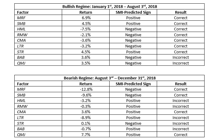
Of the five factors that the SMI predicted incorrectly during the bearish regime, three had negligible returns (RMW, STR, BAB). The biggest miss during the bearish regime was with the long-term reversal factor, LTR, which was predicted to generate positive returns but fell 8.9% instead. The biggest hit during the bearish regime was with the market factor, MRF, which fell 12.8% from August 3rd until December 31st.
SMART BUT NOT PERFECT
Despite the strong economic and statistical performance of the SMI, it is not without its limitations. There have been multiple instances in which Smart Money institutions were on the wrong side of the trade, including recently.
- The Smart Money largely exited equities in mid-1999, but the S&P 500 did not top until March 2000, almost a full year year (and about 15% higher) after institutions had become relatively bearish on equities.
- At the market bottom in March 2009, institutions were seemingly caught by surprise by the change in GAAP accounting rules that precipitated the vigorous rally off the lows. The Smart Money was still short equities when the market bottomed and did not turn long until several weeks later—missing out on a good portion of the initial rally.
- The Smart Money was also bearish equities leading up to and well after the 2016 election. They did not turn bullish (in the aggregate) until mid-2017—again missing out on a decent rally. However, when they finally did turn bullish, the market began rising at a significantly faster rate than it had been prior to their getting long.
- The Smart Money was very long equities leading up to, during, and after the February 2018 selloff in equities. The market did recover, however, and went on to make new all-time highs in September 2018. But as the equity market was rising to those new highs, the Smart Money was selling, getting out of equities at approximately 2840 on the S&P 500 in early August, about 6 weeks before the eventual all-time high.
- While up-to-date COT data has been delayed due to the recent government shutdown, as of December 31st, the Smart Money had not yet bought the dip. If that stance persists as the delayed data gradually catches up, the Smart Money will have missed out on the entirety of this most recent rally. (Notably, the Smart Money also missed out on a 20% rally in October-November 2008.)
So, as one can see, the Smart Money Indicator’s timing ability has proven imperfect over discrete intervals. In general, however, it does appear that institutions, as measured by the SMI, tend to do reasonably well at identifying the broad market trends that play out over intermediate time horizons.
Conclusion
We construct a real-time, cross-asset, positions-based relative sentiment indicator that measures how institutions are positioned in equities (and closely related assets) relative to individual investors. Upon application of a wide array of statistical tests, including ones that control for data snooping, we find the indicator appears to exhibit:
- Highly significant and exceptionally robust market timing ability
- The ability to time time-series momentum (particularly negative time-series momentum)
- The ability to time fundamentally-based smart beta equity factors
- More efficient predictive power than either value or momentum from a TAA perspective
- The potential to select equities from along a cross-section
- Out-of-sample results that are consistent with in-sample results
The SMI’s performance, although perhaps extreme in many respects, is consistent with numerous prior studies that show institutions routinely outperform individuals over intermediate time horizons. It is also consistent with the study of de Roon et al., which notes the effect of cross-hedging pressure on futures risk premia.
Taken together, past and present results lead us to the seemingly inescapable conclusion: If you want Smart Beta, it may pay to follow the Smart Money. Or as the old adage advises, “The race is not always to the swift, nor the battle to the strong, but that’s the way to bet.”
References[+]
| ↑1 | (Note: The views expressed below are solely those of the author. Thus, the term “we” in what follows should be interpreted to mean the author alone or the author and reader, depending on the context.) |
|---|---|
| ↑2 | Schmeling, Maik, 2007, Institutional and individual sentiment: Smart money and noise trader risk?, International Journal of Forecasting 23, 127–145. |
| ↑3 | Grinblatt, Mark, and Matti Keloharju, 2000, The investment behavior and performance of various investor types: a study of Finland’s unique data set, Journal of Financial Economics 55, 43–67. |
| ↑4 | Gibson, Scott, and Assem Safieddine, 2003, Does smart money move markets?, The Journal of Portfolio Management 29, 66–77. |
| ↑5 | Gibson, Scott, Assem Safieddine, and Ramana Sonti, 2004, Smart investments by smart money: Evidence from seasoned equity offerings, Journal of Financial Economics 72, 581–604. |
| ↑6 | See here for and example of research on the topic. |
| ↑7 | Asness, Clifford, 2016, The siren song of factor timing aka “smart beta timing” aka “style timing”, The Journal of Portfolio Management 42, 1–6. |
| ↑8 | Asness, Clifford, Swati Chandra, Antti Ilmanen, and Ronen Israel, 2017a, Contrarian factor timing is deceptively difficult, The Journal of Portfolio Management 43, 72–87. |
| ↑9 | de Roon, Frans Al, Theo E. Nijman, and Chris Veld, 2000, Hedging pressure effects in futures markets, The Journal of Finance 55, 1437-1456 |
| ↑10 | (Note: We orient the tests to measure the timing significance of going long the factor when the SMI is positive and we take the p-value to be the probability of observing a t-stat (or z-stat) less than the one observed. In this way, p-values near 1 indicate positive factor timing skill (i.e., factor returns are significantly better when the SMI is positive), while p-values near 0 indicate negative factor timing skill (i.e, factor returns are significantly worse when the SMI is positive).) |
| ↑11 | Romano, Joseph P., and Michael Wolf, 2005, Stepwise multiple testing as formalized data snooping, Econometrica 73, 1237–1282. |
| ↑12 | Romano, Joseph P., Azeem M. Shaikh, and Michael Wolf, 2008, Formalized data snooping based on generalized error rates, Econometric Theory 24, 404–447. |
| ↑13 | de Prado, Marcos López, and Michael J. Lewis, 2018, What is the optimal significance level for investment strategies?, SSRN Electronic Journal, URL: https://ssrn.com/abstract=3193697. |
| ↑14 | Faber, Mebane, 2007, A quantitative approach to tactical asset allocation, Journal of Wealth Management 9, 69–79. |
| ↑15 | Keller, Wouter J., and Hugo S. van Putten, 2012, Generalized momentum and flexible asset allocation (faa): An heuristic approach, SSRN Electronic Journal, URL: https://ssrn.com/abstract=2193735. |
| ↑16 | Asness, Cliff, Antti Ilmanen, and Thomas Maloney, 2015, Back in the hunt, Institutional Investor. |
| ↑17 | Keller, Wouter J. and Keuning, Jan Willem, Breadth Momentum and the Canary Universe: Defensive Asset Allocation (DAA) (July 12, 2018). Available at SSRN: https://ssrn.com/abstract=3212862 |
| ↑18 | Bilello, Charles and Gayed, Michael, Lumber: Worth It’s Weight in Gold Offense and Defense in Active Portfolio Management (May 8, 2015). 2015 NAAIM Wagner Award Winner. Available at SSRN: https://ssrn.com/abstract=2604248 |
| ↑19 | Gayed, Michael and Bilello, Charles, An Intermarket Approach to Tactical Risk Rotation: Using the Signaling Power of Treasuries to Generate Alpha and Enhance Asset Allocation (February 28, 2014). 2014 Wagner Award, 3rd Place. Available at SSRN: https://ssrn.com/abstract=2431022 |
| ↑20 | Bilello, Charles and Gayed, Michael, An Intermarket Approach to Beta Rotation: The Strategy, Signal, and Power of Utilities (January 31, 2014). 2014 Charles H. Dow Award Winner. Available at SSRN: https://ssrn.com/abstract=2417974 |
About the Author: Raymond Micaletti
—
Important Disclosures
For informational and educational purposes only and should not be construed as specific investment, accounting, legal, or tax advice. Certain information is deemed to be reliable, but its accuracy and completeness cannot be guaranteed. Third party information may become outdated or otherwise superseded without notice. Neither the Securities and Exchange Commission (SEC) nor any other federal or state agency has approved, determined the accuracy, or confirmed the adequacy of this article.
The views and opinions expressed herein are those of the author and do not necessarily reflect the views of Alpha Architect, its affiliates or its employees. Our full disclosures are available here. Definitions of common statistics used in our analysis are available here (towards the bottom).
Join thousands of other readers and subscribe to our blog.