1. Introduction
Two previous articles, “Trend-Following Filters – Part 7” [1] and “Trend-Following Filters – Part 9” [2], examined, from a digital signal processing (DSP) time domain perspective, digital filters commonly used by technical analysts to aid in making trading decisions.
- The filters examined in “Part 7” include moving average (MA), linear weighted moving average (LWMA), and exponential smoothing (ES), which are low pass filters modeled on the assumption that the input follows a first order time series process, i.e., one that has a locally constant mean value a and is contaminated with normally distributed random noise ε(t) where ε(t) ~ N(0, σε2). These filters are designed to estimate the mean value a of the input by attenuating the random noise ε(t) and were analyzed in the DSP frequency domain in “An Introduction to Digital Signal Processing for Trend Following” [3].
- The filters examined in “Part 9” include double moving average (DMA), double linear weighted moving average (DLWMA), and double exponential smoothing (DES), which are also low pass filters but are modeled on the assumption that the input follows a second order time series process, i.e., one that has a locally constant mean value a and a linear trend b which is contaminated with random normally distributed noise. These filters are designed to estimate the mean value a and linear trend b of the input by attenuating the random noise ε(t) and were analyzed in the frequency domain in “Trend-Following Filters – Part 1/2” [4]. The second order process mean regression (SOMR) filter is also included. SOMR is a low pass filter based on a second order process time series regression model and was analyzed in the frequency domain in “Trend-Following Filters – Part 8” [5].
This article examines, also from a time domain perspective, several low pass filters modeled on the assumption that the input follows a third order time series process. A third order process consists of a mean a, a linear trend b, and a quadratic trend c which is contaminated with random normally distributed noise ε(t):
third order process – mean a, linear trend b, and quadratic trend c: x(t) = a + b*t + ½*c*t2 + ε(t)
These filters are designed to estimate the mean value a, linear trend b, and quadratic trend c of the input by attenuating the random noise ε(t). Among the filters examined are:
- triple moving average (TMA) mean filter
- triple linear weighted moving average (TLWMA) mean filter
- triple exponential smoothing (TES) mean filter.
These filters were previously analyzed from a frequency domain perspective in “Trend-Following Filters – Part 2/2” [6]. The third order process mean regression (TOMR) filter is also included in the analysis. TOMR is a low pass filter based on a third order process time series regression model and was analyzed in the frequency domain in [5].
As discussed in [1], the outputs of low pass filters modeled on a first order process exhibit lag, or time delay, relative to the input if the input contains a trend. Since financial time series typically contain trends, these filters can have limited usefulness in identifying the beginning and ending of trends on a timely basis. Filters modeled on second, third, or higher order processes are, by design, better able to track trends and are commonly referred to in the technical analysis literature as “zero lag” filters.
In this article, the four third order low pass filters are examined using several time response specifications, including ones used in control system engineering [7]. The specifications are grouped into transient response and steady-state response categories:
- Transient response is defined as the temporary behavior of a system or filter after a change in the input that affects its equilibrium condition.
- Steady-state response is defined as the behavior of a system or filter when it is in an equilibrium condition. Steady-state occurs after all transient effects have subsided and the system or filter has settled into a stable state.
The specifications included are:
- transient response – delay time, rise time, peak time, peak overshoot, settling time, and trend reversal time
- steady-state response – lag, unit ramp steady-state error, unit quadratic parabola steady-state error, and unit cubic parabola steady-state error.
Technical analysts are interested in the ability of indicators not only to rapidly respond to changes in trend direction but also to minimize noise that can result in “whipsaw” trading losses. So, in addition to these specifications, variance reduction ratio (VRR), a measure of noise rejection, is included.
The time domain specifications are described in Section 4 below. The specification equations for each filter can be found in the respective appendices. In Section 5, the filter specifications and VRR are shown graphically and compared, illustrating the inherent trade-off between filter responsiveness and noise minimization. Finally, the third order filter specifications are compared on an equivalent basis to those of the first and second order filters mentioned above.
2. Note on Underlying Concepts
The characteristics of financial time series, along with the concepts of time domain and frequency domain, finite impulse response (FIR) and infinite impulse response (IIR) filters, low pass filters, difference equations, unit pulse response, and related topics, are discussed in [3]. In addition, the various inputs used to determine the filter specifications are described in [1] and [2], including unit step, unit ramp, etc., and trend reversal.
This article assumes familiarity with these concepts.
3. Overview of the Filters
This section provides brief overviews of the four filters analyzed in this article.
Triple Moving Average (TMA) Mean Filter
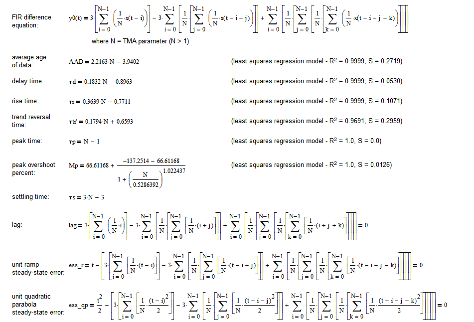
The triple moving average (TMA) mean filter is a time series forecasting and process control method that uses three single moving averages to estimate the mean of time series that contain linear and quadratic trends, as defined by Brown in [8]. (See [3] for more details regarding the single moving average.) The TMA mean filter FIR difference equation is:

where the parameter N (N > 1) is the length of the three single moving averages used to calculate the triple moving average and x(t) represents the input at integer time t. See [6] for additional details of the TMA mean filter, including the derivation of the difference equation.
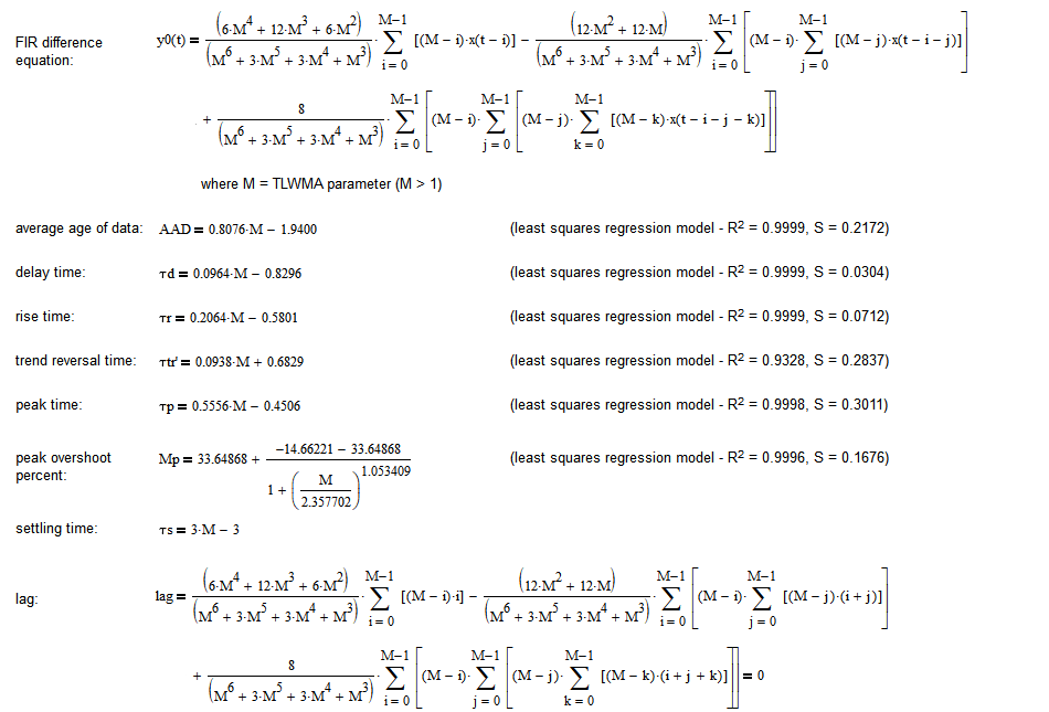
Triple Linear Weighted Moving Average (TLWMA) Mean Filter
The triple linear weighted moving average (TLWMA) mean filter is a modified form of the triple moving average which uses three single linear weighted moving averages instead of three single moving averages to estimate the mean. (See [3] for more details regarding the single linear weighted moving average.) The TLWMA mean filter FIR difference equation is:
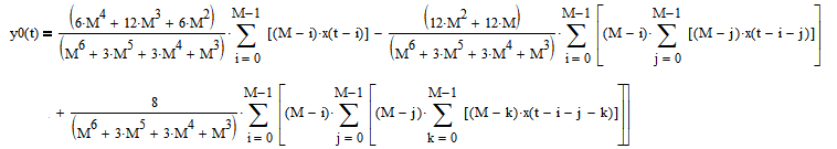
where the parameter M (M > 1) is the length of the three single linear weighted moving averages used to calculate the triple linear weighted moving average and x(t) represents the input at integer time t. See [6] for additional details of the TLWMA mean filter, including the derivation of the difference equation.
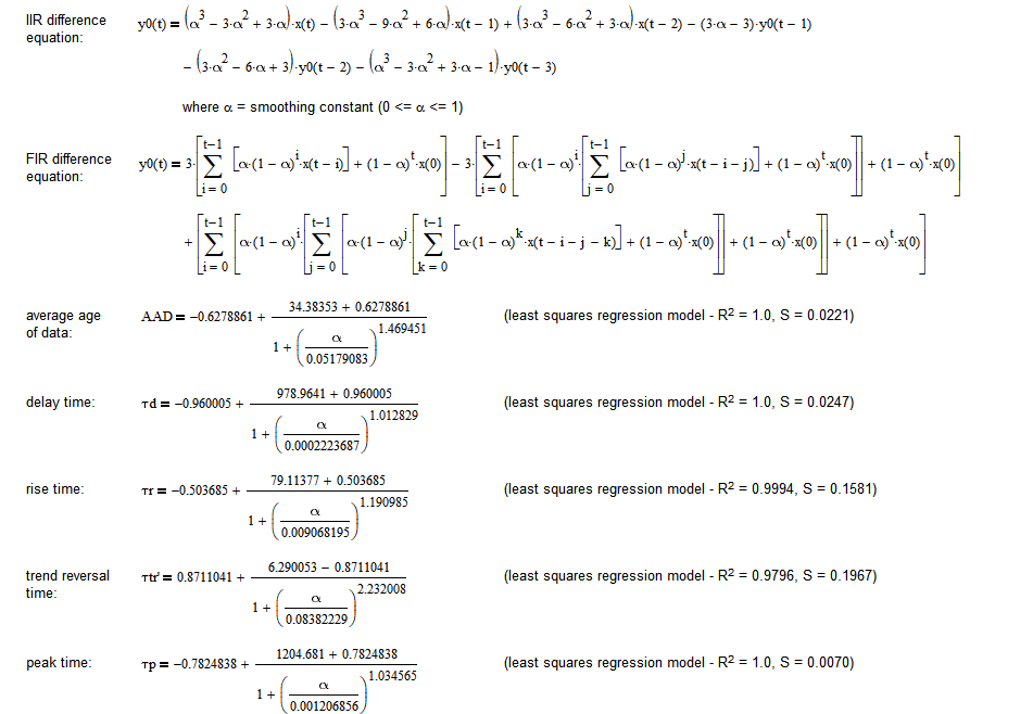
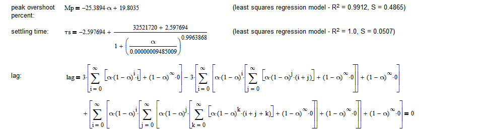
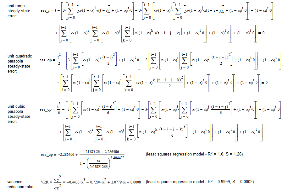
Triple Exponential Smoothing (TES) Mean Filter
The triple exponential smoothing (TES) mean filter is similar to the triple moving average, except that it uses three single exponential smoothings instead of three single moving averages to estimate the mean, as defined by Brown in [8]. The TES mean filter IIR difference equation is:
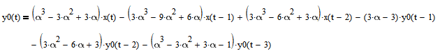
where the parameter α (0 <= α <= 1) is the exponential smoothing constant of the three single exponential smoothings used to calculate the triple exponential smoothing and x(t) represents the input at integer time t. (See [3] for more details regarding single exponential smoothing.) The corresponding FIR difference equation is:
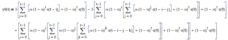
See [6] for additional details of the TES mean filter, including the derivation of the difference equation.
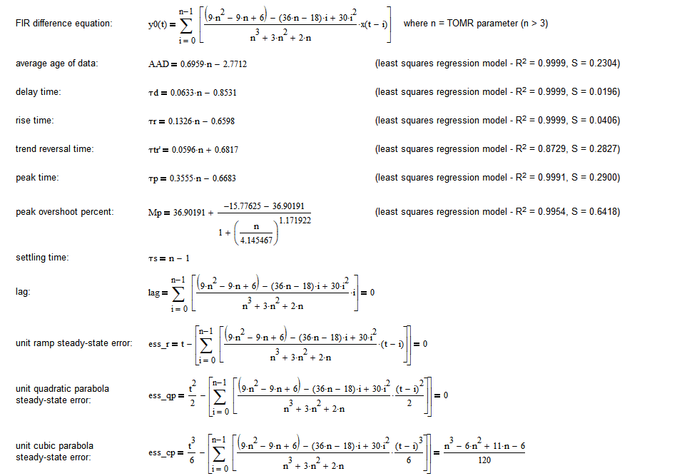
Third Order Process Mean Regression (TOMR) Filter
Section 6 of [5] shows the derivation of the third order process mean regression (TOMR) filter FIR difference equation, which is:
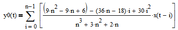
where the parameter n (n > 3) is the filter length and x(t) represents the input at integer time t.
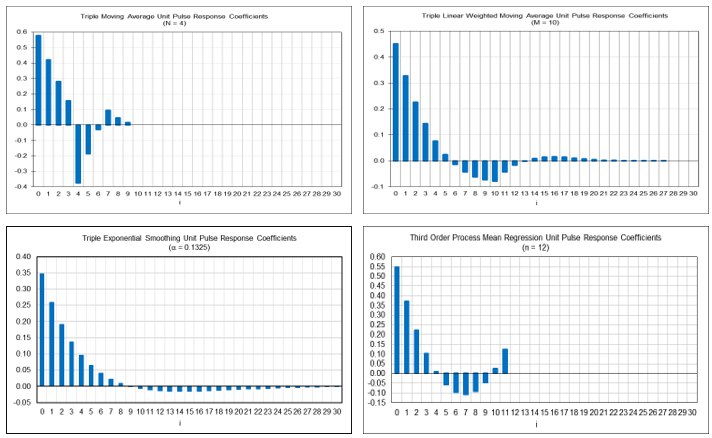
Example Filter Unit Pulse Response Coefficients
The graphs below show representative examples of the unit pulse response coefficients h(i) of the four filters, using the indicated parameter values, i.e., TMA parameter N = 4, TLWMA parameter M = 10, TES smoothing constant α = 0.1325, and TOMR parameter n = 12, with the TES coefficients displayed limited to the first 31.
4. Filter Time Domain Specifications
This section lists and briefly describes the filter time domain specifications used in this article. More detailed definitions of the specifications and of the unit inputs used can be found in [1] and [2]. The specification equations for each of the filters can be found in the respective appendices.
Note: Due to the complexity of the third order filter difference equations, it is difficult to derive closed-form analytic equations as functions of the filter parameters for many of the specifications. As an alternative, a number of the specification equations that appear in the appendices were determined by applying least squares regression to a series of measurements of the filter responses to the inputs across a wide range of parameter values. All of the resulting regression models have coefficients of determination R2 very close to 1 and small standard errors of estimate S, as indicated in the appendices.
4.1 Transient Response Specifications
Delay Time
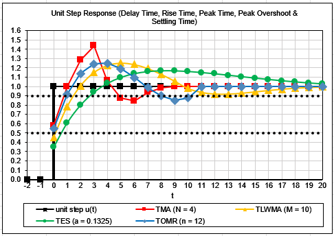
Delay time τd is measured as the number of time steps, starting at t = 0, required for the filter output to rise from 0% to 50% (0.5) of its final steady-state value in response to a unit step input. The graph below illustrates the delay times of the four filters, using the example filter parameter values. The delay time is observed when the filter output reaches the 0.5 level.
Note: The markers in the following specification graphs indicate the discrete values at each integer time t. The connecting lines have been added for visual enhancement and do not represent continuous values.
Rise Time
Rise time τr is measured as the number of time steps, starting at t = 0, required for the filter output to rise from 0% to 90% (0.9) of its final steady-state value in response to a unit step input. The graph above illustrates the rise times of the four filters, using the example filter parameter values. The rise time is observed when the filter output reaches the 0.9 level.
Peak Time
Peaking occurs during filter transient response if the filter design results in underdamping, in which case the output overshoots the final steady-state value and possibly oscillates, with the overshoot or oscillation gradually decreasing as it approaches the final steady-state value. The transient responses of the four third order filters analyzed in this article are all underdamped. See [2] for descriptions of the different types of filter damping response.
Peak time τp is measured as the number of time steps, starting at t = 0, for the filter output to reach its maximum peak value before settling at the final steady-state value in response to a unit step input. The unit step response graph above illustrates the peak times of the four filters, using the example filter parameter values.
Peak Overshoot
Peak overshoot Mp is measured as the percentage difference between the maximum peak value and the final steady-state value in response to a unit step input. The unit step response graph above illustrates the peak overshoot of the four filters, using the example filter parameter values, which occurs at their respective peak times.
Settling Time
Settling time τs is measured as the number of time steps, starting at t = 0, required for the filter output to reach and remain at the final steady-state value or, in some cases, within a specified tolerance of the final steady-state value, in response to a unit step input. In general, settling time is the number of time steps until the unit step input has reached all the filter coefficients.
The unit step response graph above illustrates the settling times of the four filters, using the example filter parameter values. For the TMA, TLWMA, and TOMR filters, settling time is observed when the filter output reaches the 1.0 level following the peak. Since the TES filter has an infinite unit step transient response time, settling time is considered here to occur when the output is within 1% of its steady-state value following the peak, i.e., at the 1.01 level.
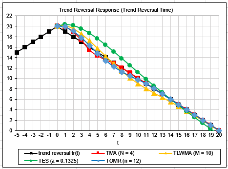
Trend Reversal Time
As discussed in [2], trend reversal time ttr’ is measured as the number of time steps between the time of the trend reversal function input peak at t = 0 and the time at which the filter output reverses direction following its own peak. The graph below illustrates the trend reversal times of the four filters, using the example filter parameter values. Note that using a trend reversal function input with slopes other than +1 and -1 results in the same relative filter responses.
4.2 Steady-State Response Specifications
Lag
Lag, the time delay of the filter output relative to the filter input, is typically measured by the response of a filter to a unit ramp input, once the filter output has reached a steady-state condition. As shown graphically below, for the TMA, TLWMA, and TOMR filters, in response to a unit ramp input, lag is zero, starting at steady-state, i.e., settling time. For the TES filter, lag asymptotically approaches zero as t increases. Note that using a ramp input with a slope other than +1 results in the same relative filter responses.
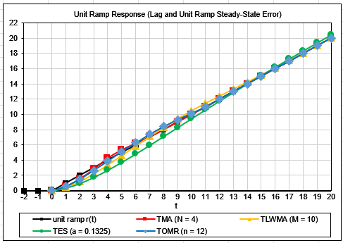
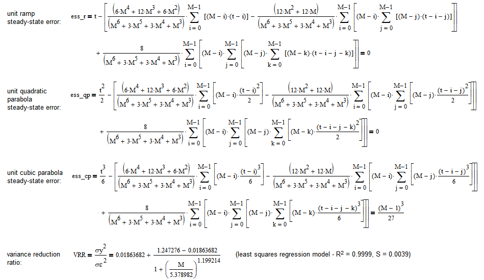
Unit Ramp Steady-State Error
Steady-state error ess is defined in general as the difference between the input x(t) and output y(t) of a system or filter when the output has reached steady-state in response to a unit input. Different unit inputs are used to measure different types of steady-state error. For example, unit ramp steady-state error ess_r measures the difference between the filter input and output in response to a unit ramp input when the filter has reached steady-state at settling time.
As shown in the graph above, for the TMA, TLWMA, and TOMR filters, the unit ramp steady-state error ess_r equals zero, starting at settling time. For the TES filter, the unit ramp steady-state error asymptotically approaches zero as t increases. Note that using a ramp input with a slope other than +1 results in the same relative filter responses.
Unit Quadratic Parabola Steady-State Error
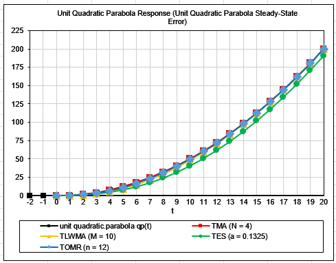
Unit quadratic parabola steady-state error ess_qp measures the difference between the filter input and output in response to a unit quadratic parabola input when the filter response reaches steady-state at settling time. As shown in the graph below, for the TMA, TLWMA, and TOMR filters, the unit quadratic parabola steady-state error ess_qp equals zero, starting at settling time. For the TES filter, the unit quadratic parabola steady-state error asymptotically approaches zero as t increases. Note that using a quadratic parabola input with a coefficient other than ½ results in the same relative filter responses.
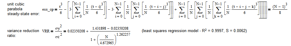
Unit Cubic Parabola Steady-State Error
An additional specification, unit cubic parabola steady-state error ess_cp measures the difference between the filter input and output in response to a unit cubic parabola input when the filter response reaches steady-state at settling time. The unit cubic parabola input is based on a third-degree cubic polynomial function and is denoted by cp(t) where:
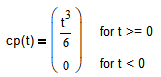
The unit cubic parabola function is illustrated in the following graph.
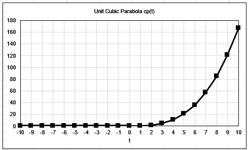
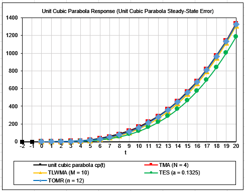
As shown in the graph below, for the four filters, the unit cubic parabola steady-state error is non-zero but constant and is a function of the filter parameter value. Note that using a cubic parabola input with a coefficient other than 1/6 results in the same relative filter responses.
4.3 Variance Reduction Ratio
For time series containing normally distributed random noise ε(t), the variance reduction ratio (VRR) of a filter measures the reduction in the variance σy2 of the filter output y(t) relative to the variance σε2 of the filter input x(t). The smaller the ratio σy2/σε2, the greater the noise reduction. For example, VRR = 0 indicates complete noise reduction, whereas VRR = 1 indicates no noise reduction.
5. Filter Specification Comparison
In general, for low pass filters modeled on a third order process:
- The speed with which a filter responds to a change in the input can be measured by delay time, rise time, settling time, and trend reversal time.
- Filter tracking error, i.e., how closely the filter output follows the input, can be measured by peak time, peak overshoot, lag, unit ramp steady-state error, unit quadratic parabola steady-state error, and unit cubic parabola steady-state error.
- Filter noise rejection can be measured by the variance reduction ratio (VRR).
The following graphs show the transient response specifications and VRR of the four third order filters across a range of filter parameter values.
The graphs indicate that, in general, the larger the filter parameters N, M, and n, or the smaller the smoothing constant α, the smaller the VRR but also the greater the delay time, rise time, peak time, peak overshoot, settling time, and trend reversal time.
In order for the specifications to be comparable across the filters, the filter parameter values need to be standardized. As discussed in [1] and [2], an important metric for analyzing and comparing the time domain characteristics of filters is the average age of the data (AAD) passing through them, as defined by Brown in [8]. The graphs below show the AADs of the four filters across a range of parameter values. The AAD equations are shown in the respective appendices.
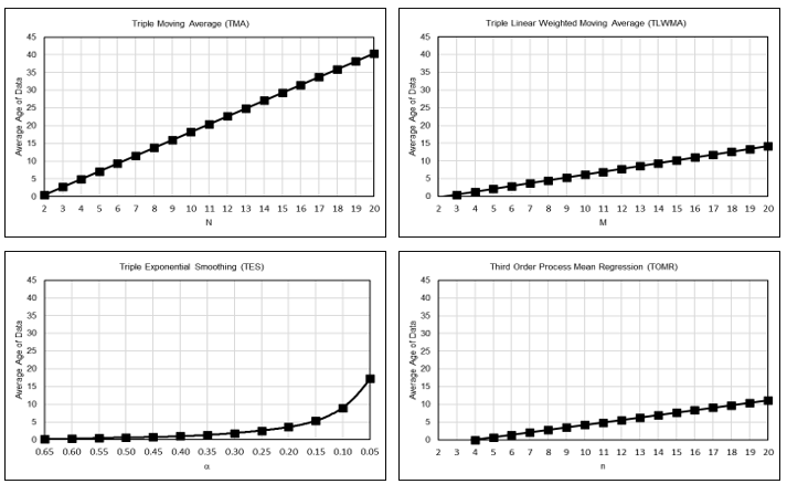
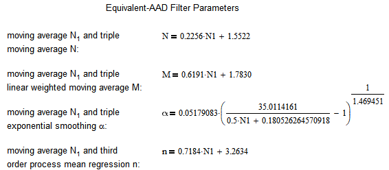
Since AAD is commonly used in the technical analysis literature to calculate equivalent filter parameters, the method chosen here is to convert the parameters values to the corresponding single moving average filter length, denoted by N1, so they have equivalent AAD. The filter parameter conversion equations are shown below.
The graphs below show the transient response specifications and VRR for the four filters, standardized on the corresponding equivalent-AAD single moving average filter length N1.
The graphs indicate that:
- TMA has the shortest delay time, rise time, peak time, settling time, and trend reversal time but the largest peak overshoot and the highest VRR.
- TOMR has the shortest trend reversal time, but TMA is only slightly longer.
- TES has the longest delay time, rise time, peak time, settling time, and trend reversal time but the smallest peak overshoot and the lowest VRR.
The following table compares the transient response specifications and VRR on an equivalent-AAD basis across the three low pass filters modeled on a first order process as discussed in [1], the four low pass filters modeled on a second order process as discussed in [2], and the four low pass filters modeled on a third order process as discussed in this article. The individual specifications of each filter are ranked from 1 to 11, where 1 indicates the shortest/smallest and 11 indicates the longest/largest. Note that, as discussed in [5], the equation for the first order process mean regression filter is the same as for the single moving average filter, so the first order process mean regression filter is not included here.
The filters can be ranked overall, for example, by applying weights, where the weights add up to 1.0, to each of the individual specifications according to their relative importance and summing to arrive at a total score for each filter. The trade-off between trend reversal time and variance reduction ratio is typically the most relevant to consider in filter selection and design with regard to trading applications.
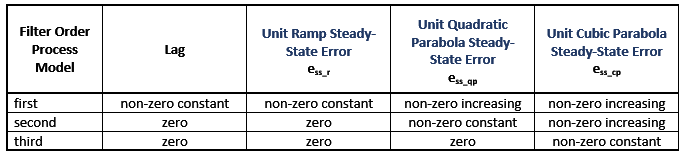
The following table qualitatively indicates the steady-state error responses for all the filter types, based on the process model on which they are designed.
6. Comments
In summary:
- As discussed in [1], low pass filters modeled on a first order process, such as MA, LWMA, and ES, exhibit non-zero lag and non-zero steady-state error in response to linear and higher order trends.
- As discussed in [2], low pass filters modeled on a second order process, such as DMA, DLWMA, DES, and SOMR, are often referred to as “zero lag” filters, due to their ability to track linear trends in steady-state with no lag. However, they exhibit non-zero lag and non-zero steady-state error in response to quadratic and higher order trends.
- The low pass filters modeled on a third order process discussed in this article, such as TMA, TLWMA, TES, and TOMR, are also often referred to as “zero lag” filters, due to their ability to track linear and quadratic trends in steady-state with no lag. However, they exhibit non-zero lag and non-zero steady-state error in response to cubic and higher order trends.
From a practical standpoint, all low pass filters, when operating on financial time series, are often, if not usually, in a transient state, due to the volatility and non-stationarity of those time series [3]. As a result, the output of all of these filters generally display some amount of lag for much of the time, whether they are labeled as “zero lag” or not.
Further detailed analysis regarding many of the filters discussed in these articles as well as of a number of other types of filters can be found in [9].
Appendix 1 – Triple Moving Average (TMA) Mean Filter Specifications
Appendix 2 – Triple Linear Weighted Moving Average (TLWMA) Mean Filter Specifications
Appendix 3 – Triple Exponential Smoothing (TES) Mean Filter Specifications
Appendix 4 – Third Order Process Mean Regression (TOMR) Filter Specifications

References
[1] Stern, H., “Trend-Following Filters – Part 7”, October 2023, updated: March 2025; available online at https://alphaarchitect.com/2023/10/trend-following-filters-part-7/.
[2] Stern, H., “Trend-Following Filters – Part 9”, June 19, 2025; available online at https://alphaarchitect.com/trend-following-filters-part-9/.
[3] Stern, H., “An Introduction to Digital Signal Processing for Trend Following”, August 2020, updated: March 2025; available online at https://alphaarchitect.com/2020/08/an-introduction-to-digital-signal-processing-for-trend-following/.
[4] Stern, H., “Trend-Following Filters – Part 1/2”, December 2020; available online at https://alphaarchitect.com/2020/12/29/trend-following-filters-part-1-2/.
[5] Stern, H., “Trend-Following Filters – Part 8”, September 2024; available online at https://alphaarchitect.com/2024/09/trend-following-filters-part-8/.
[6] Stern, H., “Trend-Following Filters – Part 2/2”, January 2021; available online at https://alphaarchitect.com/2021/01/21/trend-following-filters-part-2-2/.
[7] Gowda, K., “Control Systems 2.4 – Time Response Specifications”, March 2021; available online at https://www.circuitbread.com/tutorials/time-response-specifications-2.4.
[8] Brown, R. G., Smoothing, Forecasting, and Prediction of Discrete Time Series, Prentice Hall, 1962.
[9] Zakamulin, V. and Giner, J., The Ultimate Moving Average Handbook, Palgrave Macmillan, 2025.
About the Author: Henry Stern
—
Important Disclosures
For informational and educational purposes only and should not be construed as specific investment, accounting, legal, or tax advice. Certain information is deemed to be reliable, but its accuracy and completeness cannot be guaranteed. Third party information may become outdated or otherwise superseded without notice. Neither the Securities and Exchange Commission (SEC) nor any other federal or state agency has approved, determined the accuracy, or confirmed the adequacy of this article.
The views and opinions expressed herein are those of the author and do not necessarily reflect the views of Alpha Architect, its affiliates or its employees. Our full disclosures are available here. Definitions of common statistics used in our analysis are available here (towards the bottom).
Join thousands of other readers and subscribe to our blog.