1. Introduction
Many traders use strategies based on trends that occur in stock, bond, currency, commodity, and other financial asset price time series in order to “buy low” and “sell high”. A trend is considered to be the overall direction of prices over a period of time. If prices have generally increased the trend has a positive slope and is called “bullish”. If prices have generally decreased, the trend has a negative slope and is called “bearish”. If there is no discernable positive or negative trend, the trend is often referred to as “sideways”.(1)
Trend-based trading strategies include:
- momentum – trading in the same direction as the recent trend on the expectation that the trend will continue. (see here for an example)
- mean reversion – anticipating reversals from “extreme” price levels considered to be “overbought” or “oversold”
- contrarian – trading against the prevailing trend on the expectation that the trend will soon end. (see here for an example)
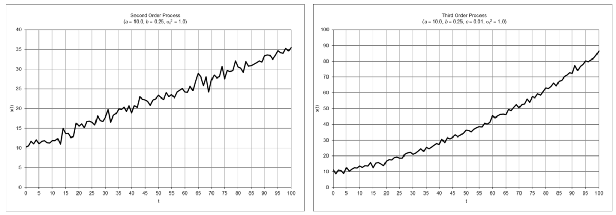
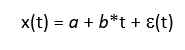
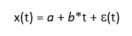
Since financial time series data are digital by nature, digital filtering techniques are used by many technical analysts to transform and analyze them, e.g., to attenuate noise and identify trends. For example, moving averages and exponential smoothing are commonly used directly and are also embedded in many technical indicators, such as moving average crossover (MAC) and moving average convergence-divergence (MACD). Moving averages and exponential smoothing are examples of low pass digital filters, which are modeled on the assumption that the input follows a first-order process, i.e., one that has a locally constant mean value a and is contaminated with normally distributed random noise ε(t) where ε(t) ~ N(0, σε2):
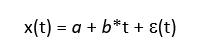
- first order process – mean a: x(t) = a + ε(t)
Low pass filters are designed to estimate the mean value α of a first-order process by attenuating the random noise ε(t). However, if the input contains trends, the output of a low pass filter will lag the input because it is not designed to model trends. While the lagged response can be used as a way to “sidestep” some of the noise and short-term price fluctuations during a trend, there is a cost of delayed response once a trend begins or ends.
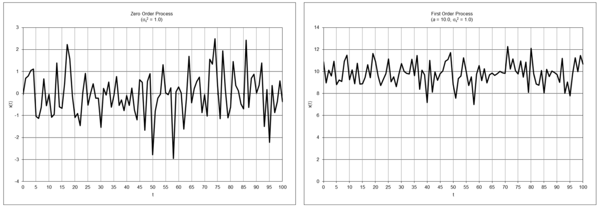
Note: A zero order process just consists of random noise, which is equivalent to a first order process with mean a = 0:
- zero order process: x(t) = ε(t)
The following graphs show examples of times series with underlying zero and first order processes:
Because financial time series typically exhibit trends, it is appropriate to use filters that are modeled on the assumption that the input follows an underlying process containing trends, for example:
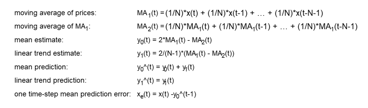
- second order process – mean a and linear trend b: x(t) = a + b*t + ε(t)
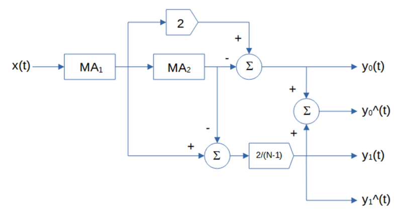
- third order process – mean a, linear trend b, and quadratic trend c: x(t) = a + b*t + ½*c*t2 + ε(t)
The following graphs show examples of times series based on underlying second and third order processes:
Part 1 of this analysis examines filters modeled on second-order processes, specifically double moving average, double linear weighted moving average, double exponential smoothing, and alpha-beta tracking filters, from a digital signal processing (DSP) perspective to illustrate their properties and limitations.
Part 2 will examine filters modeled on third-order processes, specifically triple moving average, triple linear weighted moving average, triple exponential smoothing, and alpha-beta-gamma tracking filters.
These filters are sometimes called “zero lag” filters, although they reduce but do not totally eliminate lag in all circumstances.
2. Notes on the Underlying Concepts and Graphs
- The characteristics of financial time series along with the underlying concepts of frequency and period measurement, time domain, and frequency domain, the four basic types of filters, finite impulse response (FIR) and infinite impulse response (IIR) filters, and filter frequency response are discussed in “An Introduction to Digital Signal Processing for Trend Following”, which is available on the Alpha Architect website blog here. This article assumes familiarity with that material.
- The unit pulse response graphs shown for each filter in this article display the time domain responses on the integer time scale t = 0, 1, 2, …. The coefficients of an FIR filter correspond to the time-reversed order of the unit pulse response.
- The frequency magnitude spectrum graphs shown for each filter display the frequency domain response over the normalized frequency range 0 <= f <= 0.5 cycles per time sample on the horizontal scale. The lower limit f = 0 can be thought of as a wave of infinite length or as a steady direct current (DC) level. The upper limit f = 0.5 is called the “Nyquist frequency”, which is the highest frequency of a signal that can be recorded per time sample for the signal to be accurately reconstructable in the time domain.
- Graphs showing the magnitude spectrum for each filter in terms of period P, i.e., the number of time samples to complete one cycle, on the horizontal scale are also included, since period is the measurement that is most commonly used by and familiar to technical analysts. These graphs have a lower limit of 2 time samples, since the Nyquist frequency f = 0.5 corresponds to a period of P = 1/f = 2 time samples per cycle.
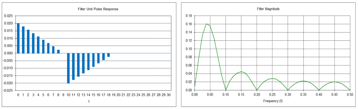
- In the frequency phase spectrum graphs shown for each filter, phase values are constrained to the range -180 to +180 degrees. When the actual phase value is outside this range, the phase value is increased or decreased by a multiple of 360 degrees to put the phase value back within the -/+ 180-degree range. This is called “phase wrap” and results in the appearance of a zig-zag line, but each 360 degree line segment jump is actually a continuation of the previous line segment.
- Examples of the time domain output of the various filters are shown using price charts of the daily S&P 500 stock index closing values for 2018 and 2019, which includes 503 trading days.
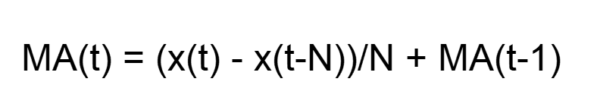
3. Double Moving Average (DMA)
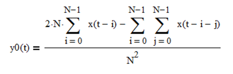
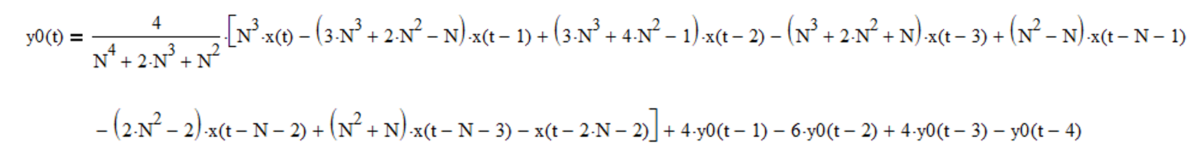
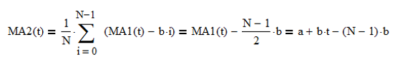
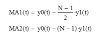
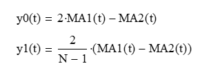
Double moving average (DMA) is a time series forecasting and process control method that uses two single moving averages to estimate the mean and trend of time series that contain linear trends(2). The double moving average set of equations is:
where N is the number of input data points, i.e., the moving average length N (N > 1), included in the two single moving averages used to calculate the double moving average, and x(t) represents the price at integer time t. The derivation of the double moving average equations is shown in Appendix 1.
The double moving average generates three main outputs: an estimate of the mean y0(t) at time step t, an estimate of the linear trend y1(t) at time step t, and a mean prediction y0^(t) made at time step t for the next time step t+1. The linear trend prediction y1^(t) for the next time step t+1 is the same as the linear trend estimate y1(t), since a double moving average does not model non-linear trends.
The single moving average (MA) equations shown above are in FIR (non-recursive) form. The filter coefficients have equal value 1/N. The IIR (recursive) form, which requires proper initialization, is:
Note that a single moving average actually has two outputs: an estimate of the mean and a mean prediction for the next time step, but the mean prediction is the same as the mean estimate, since a single moving average does not model trends.
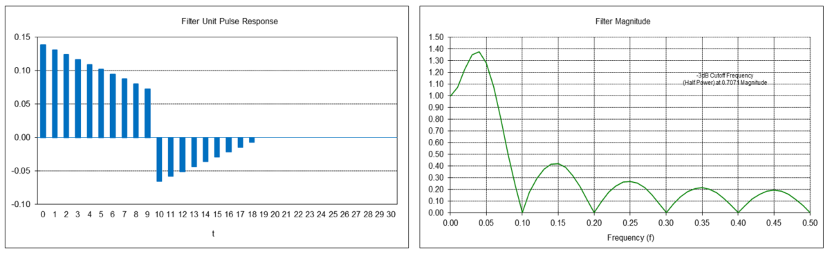
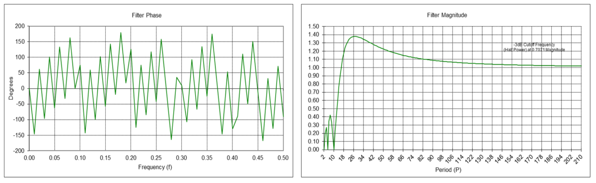
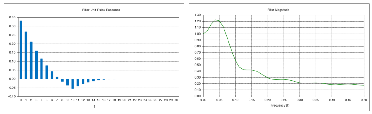
Double Moving Average Mean Filter Frequency Response (N=10)
The double moving average mean filter y0(t) is a type of FIR low pass filter, i.e., it passes frequencies below the cutoff frequency fc and attenuates frequencies above the cutoff frequency. The value N determines the cutoff frequency, which is inversely proportional to N (the cutoff period Pc is proportional to N). The filter coefficients sum to 1.0.
FIR mean filter difference equation:
IIR mean filter difference equation (requires proper initialization):

Example: Double moving average mean filter with length N = 10
Passes frequencies below the -3 dB (half power) cutoff frequency fc of approximately 0.0734, which corresponds to a cutoff period Pc of approximately 13.6 time samples. Completely suppresses frequencies of 0.1, 0.2, 0.3, 0.4, and 0.5, which correspond to periods of 10, 5, 3.3333, 2.5, and 2 time samples, respectively. (Suppression occurs because, for example, the average value of a 10 time-sample period sine wave over 10 time samples is zero, the average value of two 5 time-sample period sine waves over 10 time samples is zero, etc.) There is a magnitude peak above 1.0 (i.e., 0 dB) at a period of approximately 27 time samples.
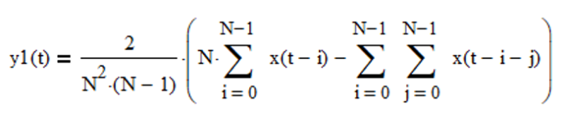
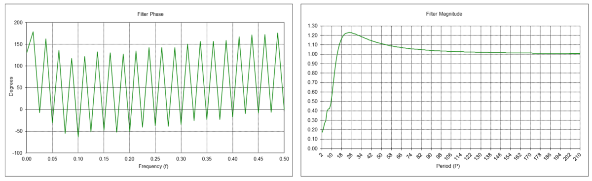
Double Moving Average Linear Trend Filter Frequency Response (N = 10)
The double moving average linear trend filter y1(t) is a type of FIR bandpass filter. The filter has a center (also called “resonant”) frequency f0, corresponding to a center period P0, which passes at maximum power. The value N determines the center frequency f0, which is inversely proportional to N (the center period P0 is proportional to N). The filter coefficients sum to 0.0.
FIR linear trend filter difference equation:
IIR linear trend filter difference equation (requires proper initialization):

Example: Double moving average linear trend filter with length N = 10
The center frequency f0 is approximately 0.0417, which corresponds to a center period P0 of approximately 24 time samples. The filter completely suppresses frequencies of 0.1, 0.2, 0.3, 0.4, and 0.5, which correspond to periods of 10, 5, 3.333, 2.5, and 2 time samples, respectively.
Double Moving Average Mean and Linear Trend Filter Example
The following S&P 500 daily price chart shows the double moving average mean (dashed blue line) and linear trend (solid blue line) for filter length N = 10. The single moving average mean (dashed red line) for filter length N = 10 is shown for comparison.
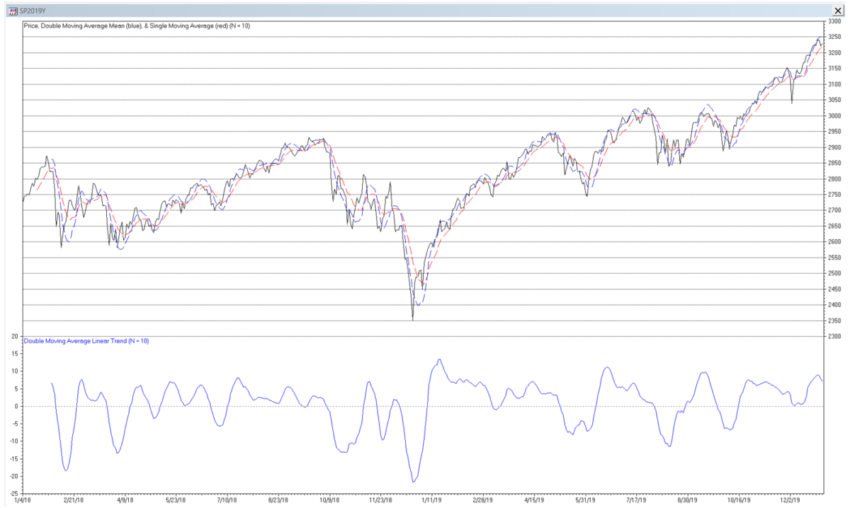
The amplitude of the linear trend filter output is proportional to the local slope of the price, i.e., the greater the amplitude, the steeper the slope, although the output can be affected by the presence of cycles and non-linear trends.
Trading Signal Generation
Trading signals using double moving average mean and linear trend filters can potentially be generated, for example, when:
- the price crosses above (buy) or below (sell) the mean line
- the mean line reaches a local crest (sell) or trough (buy)
- the linear trend line crosses above (buy) or below (sell) the zero line
- the linear trend line reaches a local crest (sell) or trough (buy)
or by a combination of these conditions.
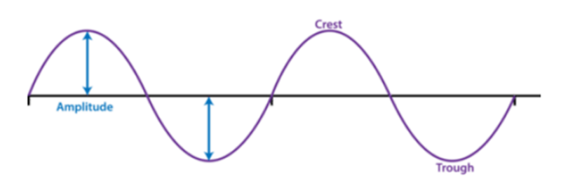
The graph below illustrates the concepts of amplitude, crest, and trough:
4. Double Linear Weighted Moving Average (DLWMA)
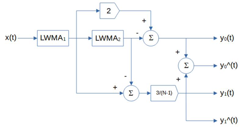
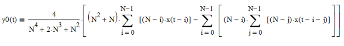
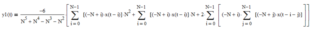
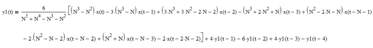
Double linear weighted moving average (DLWMA) is a modified form of double moving average that uses linear weighted moving averages instead of moving averages to estimate the mean and linear trend. The double linear weighted moving average set of equations is:
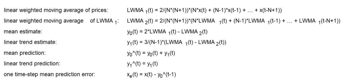
where N is the number of input data points, i.e., the linear weighted moving average length N (N > 1), included in the two single linear weighted moving averages used to calculate the double linear weighted moving average, and x(t) represents the price at integer time t. The derivation of the double linear weighted moving average equations is shown in Appendix 2.
The double linear weighted moving average generates three main outputs: an estimate of the mean y0(t) at time step t, an estimate of the linear trend y1(t) at time step t, and a mean prediction y0^(t) made at time step t for the next time step t+1. The linear trend prediction y1^(t) for the next time step t+1 is the same as the linear trend estimate y1(t), since a double linear weighted moving average does not model non-linear trends.
The single linear weighted moving average (LWMA) equations shown above are in FIR (non-recursive) form. The filter coefficients are linearly weighted with the greatest weights placed on the most recent input values. The IIR (recursive) form, which requires proper initialization, is:

Note that a single linear weighted moving average actually has two outputs: an estimate of the mean and a mean prediction for the next time step, but the mean prediction is the same as the mean estimate, since a single linear weighted moving average does not model trends.
Double Linear Weighted Moving Average Mean Filter Frequency Response (N = 10)
The double linear weighted moving average mean filter y0(t) is a type of FIR low pass filter, i.e., it passes frequencies below the cutoff frequency fc and attenuates frequencies above the cutoff frequency. The value N determines the cutoff frequency, which is inversely proportional to N (the cutoff period Pc is proportional to N). The filter coefficients sum to 1.0.
FIR mean filter difference equation:
IIR mean filter difference equation (requires proper initialization):
Example: Double linear weighted moving average mean filter with length N = 10
Passes frequencies below the -3 dB (half power) cutoff frequency fc of approximately 0.0894, which corresponds to a cutoff period Pc of approximately 11.2 time samples. There is a magnitude peak above 1.0 (i.e., 0 dB) at a period of approximately 24 time samples.
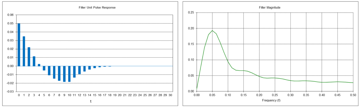
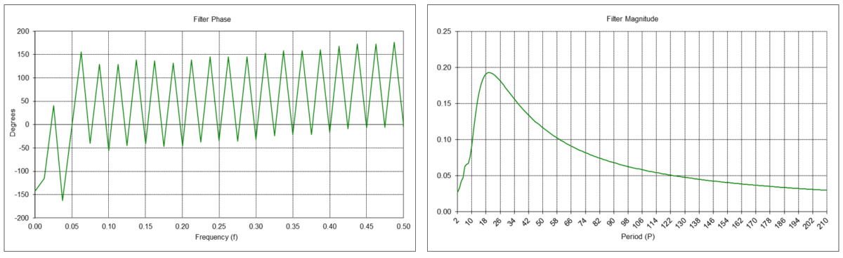
Double Linear Weighted Moving Average Linear Trend Filter Frequency Response (N = 10)
The double linear weighted moving average linear trend filter y1(t) is a type of FIR bandpass filter. The filter has a center (also called “resonant”) frequency f0, corresponding to a center period P0, which passes at maximum power. The value N determines the center frequency f0, which is inversely proportional to N (the center period P0 is proportional to N). The filter coefficients sum to 0.0.
FIR linear trend filter difference equation:
IIR linear trend filter difference equation (requires proper initialization):
Example: Double linear weighted moving average linear trend filter with length N = 10
The center frequency f0 is approximately 0.05, which corresponds to a center period P0 of approximately 20 time samples.
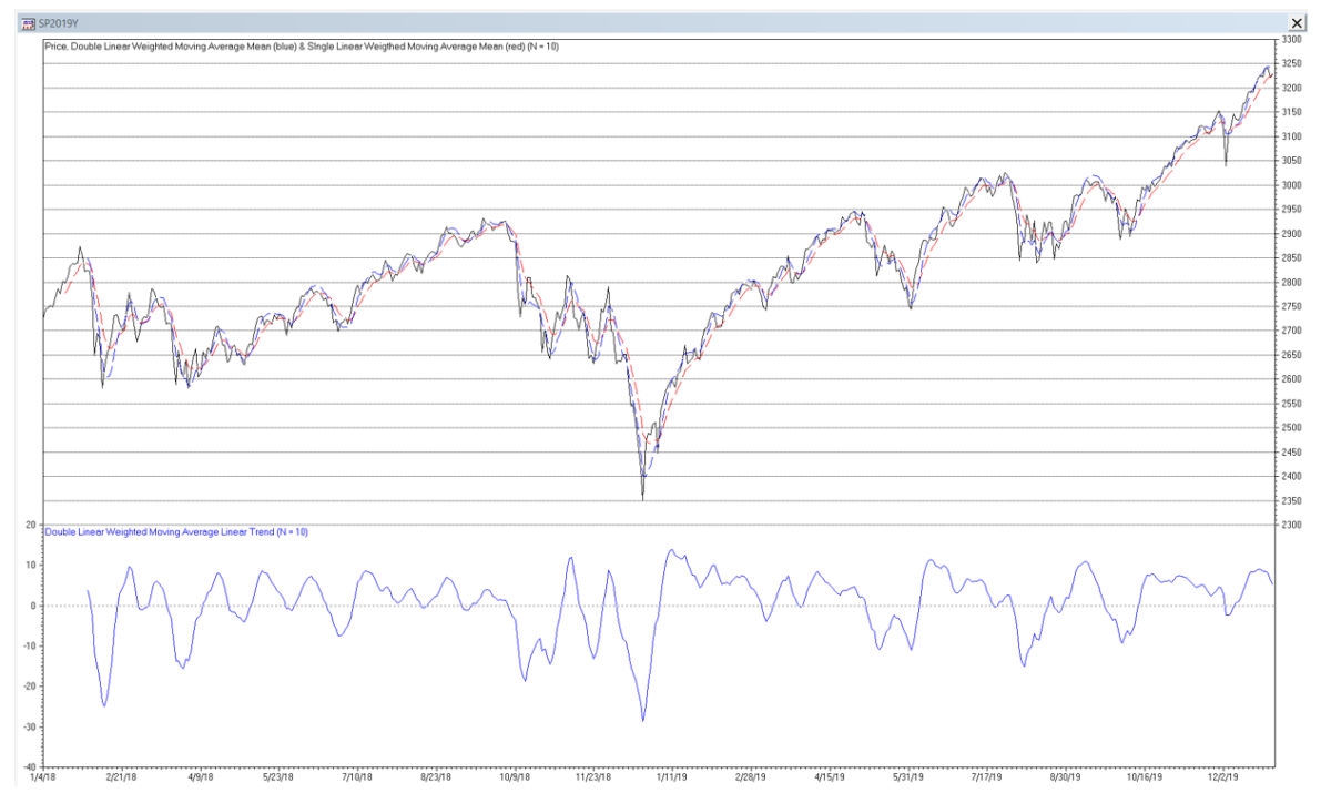
Double Linear Weighted Moving Average Mean and Linear Trend Filter Example
The following S&P 500 daily price chart shows the double linear weighted moving average mean (dashed blue line) and linear trend (solid blue line) for filter length N = 10. The single linear weighted moving average mean (dashed red line) for filter length N = 10 is shown for comparison.
Trading signals using double linear weighted moving average mean and linear trend filters can potentially be generated in a similar manner to those described for double moving average mean and linear trend filters.
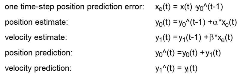
5. Double Exponential Smoothing (DES)
Double exponential smoothing (DES) is similar to the double moving average, except that it uses exponential smoothing instead of moving averages to estimate the mean and linear trend(3). The double exponential smoothing set of equations is:
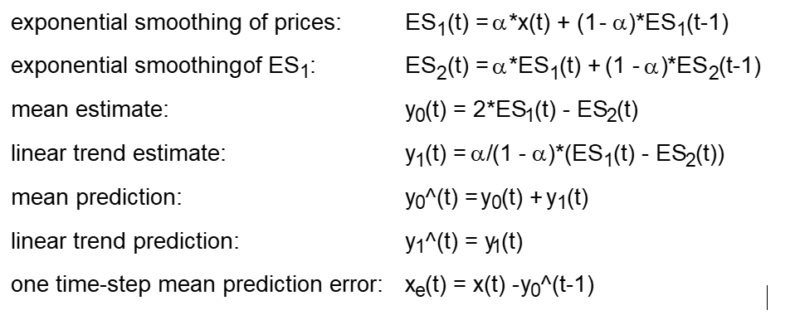
where α is the exponential smoothing constant (0 <= α <= 1) used in the two single exponential smoothings used to calculate the double exponential smoothing, and x(t) represents the price at integer time t. The derivation of the double exponential smoothing equations is shown in Appendix 3.
Double exponential smoothing generates three main outputs: an estimate of the mean y0(t) at time step t, an estimate of the linear trend y1(t) at time step t, and a mean prediction y0^(t) made at time step t for the next time step t+1. The linear trend prediction y1^(t) for the next time step t+1 is the same as the linear trend estimate y1(t), since double exponential smoothing does not model non-linear trends.
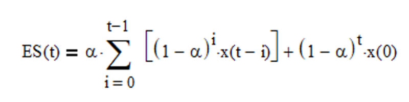
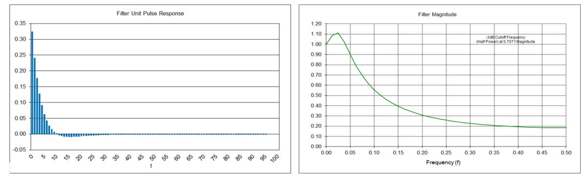
The single exponential smoothing (ES) equations shown above are in IIR (recursive) form, which requires proper initialization. The filter smoothing constant α is applied to the current input value and (1 – α) is applied to the previous filter output value. The FIR (non-recursive) form is:
Note that single exponential smoothing actually has two outputs: an estimate of the mean and a mean prediction for the next time step, but the mean prediction is the same as the mean estimate, since single exponential smoothing does not model trends.
Double Exponential Smoothing Mean Filter Frequency Response (α = 0.1772)
The double exponential smoothing mean filter y0(t) is a type of IIR low pass filter, i.e., it passes frequencies below the cutoff frequency fc and attenuates frequencies above the cutoff frequency. The value of the exponential smoothing constant α determines the cutoff frequency, which is proportional to α (the cutoff period Pc is inversely proportional to α).
IIR mean filter difference equation (requires proper initialization):

Example: Double exponential smoothing mean filter with exponential smoothing constant α = 0.1772
The filter has about the same -3 dB (half power) cutoff frequency fc of approximately 0.0734 (cutoff period Pc of approximately 13.6 time samples) as a double moving average filter with length N = 10. There is a magnitude peak above 1.0 (i.e., 0 dB) at a period of approximately 48 time samples.
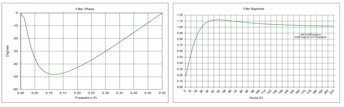
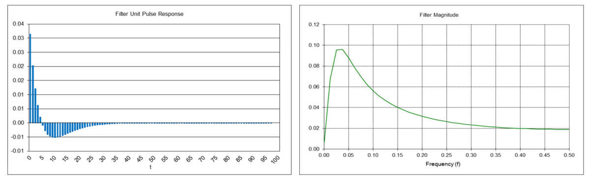
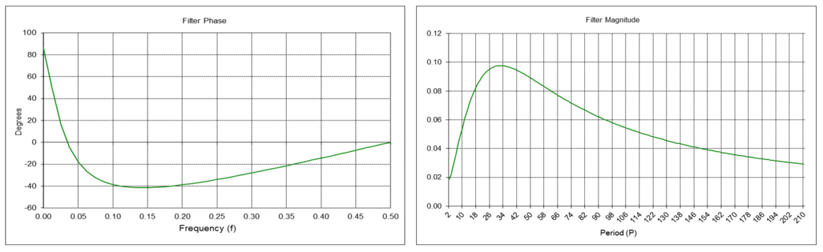
Double Exponential Smoothing Linear Trend Filter Frequency Response (α = 0.1772)
The double exponential smoothing linear trend filter y1(t) is a type of IIR bandpass filter. The filter has a center (also called “resonant”) frequency f0, corresponding to a center period P0, which passes at maximum power. The value of the exponential smoothing constant α determines the center frequency f0, which is proportional to α (the center period P0 is inversely proportional to α).
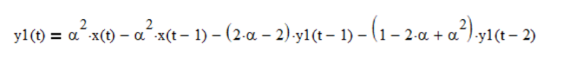
IIR linear trend filter difference equation (requires proper initialization):
Example: Double exponential smoothing linear trend filter with exponential smoothing constant α = 0.1772
The center frequency f0 is approximately 0.0313, which corresponds to a center period P0 of approximately 32 time samples.
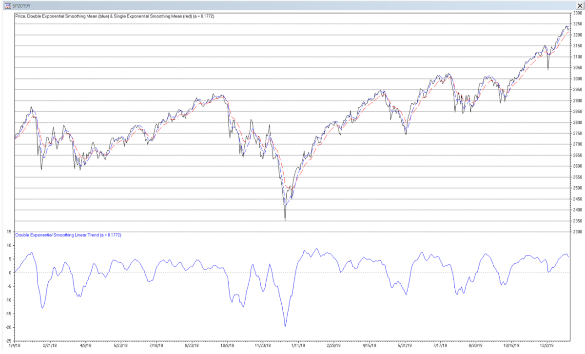
Double Exponential Smoothing Mean and Linear Trend Filter Example
The following S&P 500 daily price chart shows the double exponential smoothing mean (dashed blue line) and linear trend (solid blue line) with smoothing constant α = 0.1772. The single exponential smoothing mean (dashed red line) with smoothing constant α = 0.1772 is shown for comparison.
Trading signals using double exponential smoothing mean and linear trend filters can potentially be generated in a similar manner to those described for double moving average mean and linear trend filters.
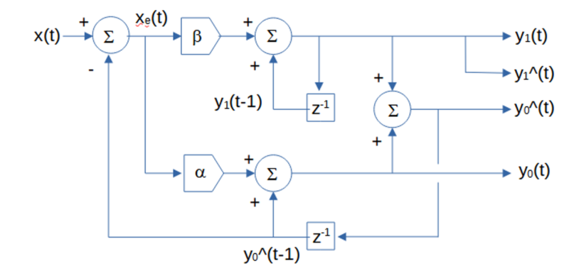
6. Alpha-Beta (α-β) Tracking Filter
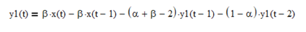
The alpha-beta (α-β) filter is used for object tracking in track-while-scan radar systems, based on a linear motion model(4). The function of the tracking filter is to process noisy position measurement inputs into “smoothed” position and velocity estimate outputs. The alpha-beta tracking filter set of equations is:
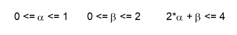
where α is the position smoothing constant, β is the velocity smoothing constant, and x(t) is the observed position of the object (or price in this case) at integer time t. Note that the alpha-beta filter position estimate is analogous to the mean estimate and the velocity estimate is analogous to the linear trend estimate of the other filters described above. The α and β smoothing constants are subject to the following stability constraints:
The alpha-beta tracking filter generates three main outputs: an estimate of the position y0(t) at time step t, an estimate of the velocity y1(t) at time step t, and a position prediction y0^(t) made at time step t for the next time step t+1. The velocity prediction y1^(t) for the next time step t+1 is the same as the velocity estimate y1(t), since the alpha-beta tracking filter does not model acceleration and higher order maneuvers.
Various alpha-beta filter smoothing constant relationship equations have been developed to calculate optimal values, based on an assumed underlying process model that approximates the dynamic behavior of the target or on a set of filter design objectives, such as providing good transient response and small noise and prediction error (5) (6). They include:
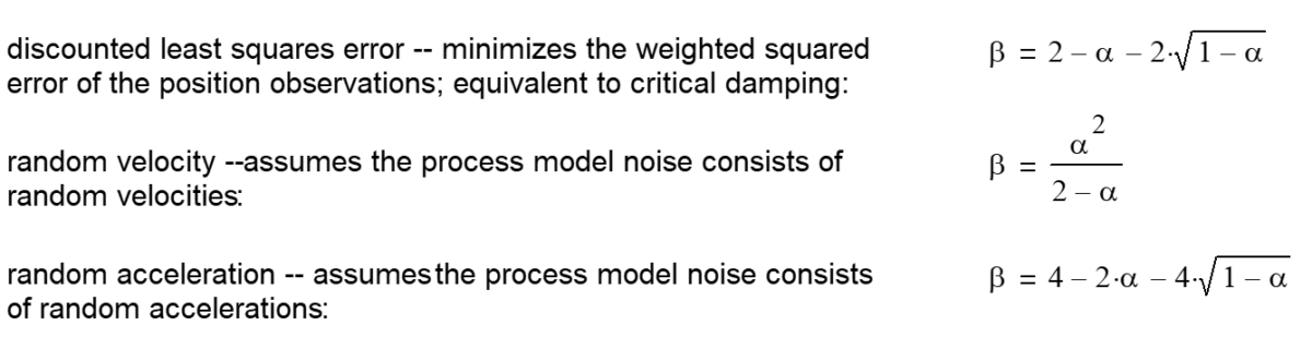
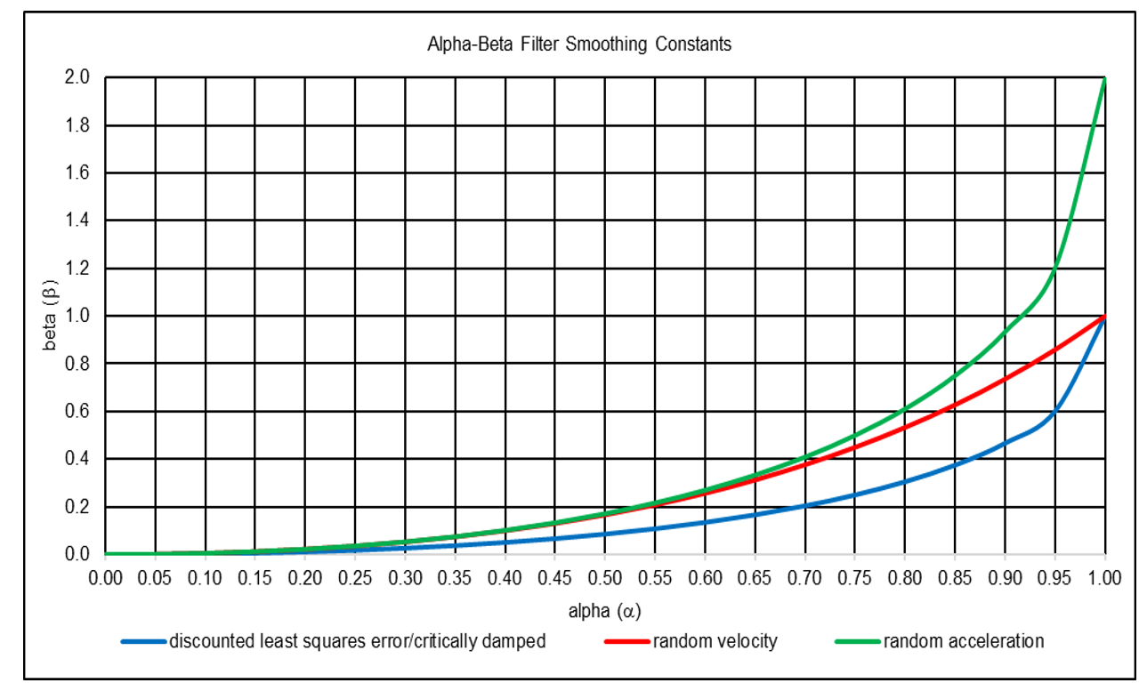
Notes:
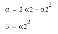
- Discounted least squares error (critically damped) smoothing constants α and β produce results equivalent to double exponential smoothing if
- The alpha tracking filter, which only estimates position, is comparable to single exponential smoothing and is closely related to the one-state steady-state Kalman filter, where the single state is position. Similarly, the alpha-beta tracking filter is closely related to the two-state steady-state Kalman filter, where the two states are position and velocity(7).
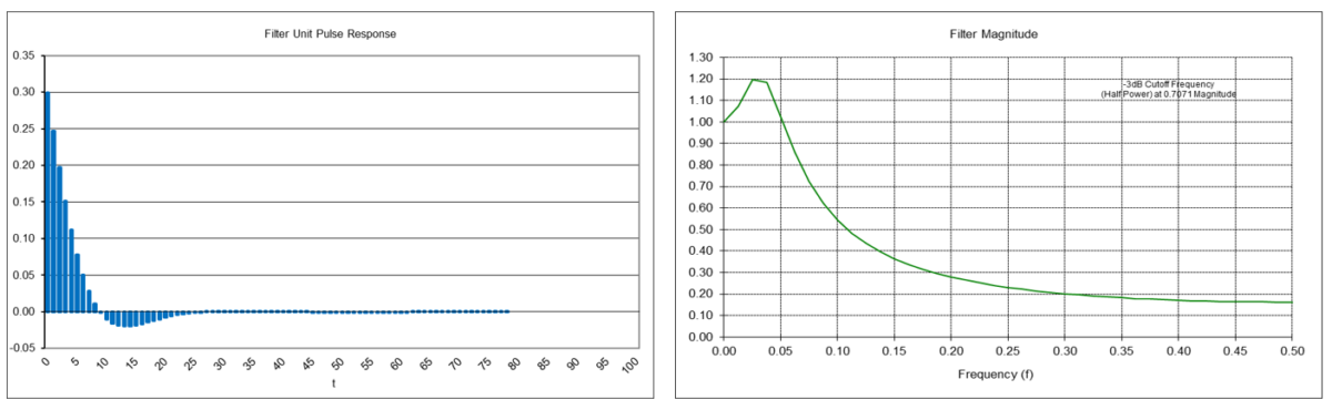
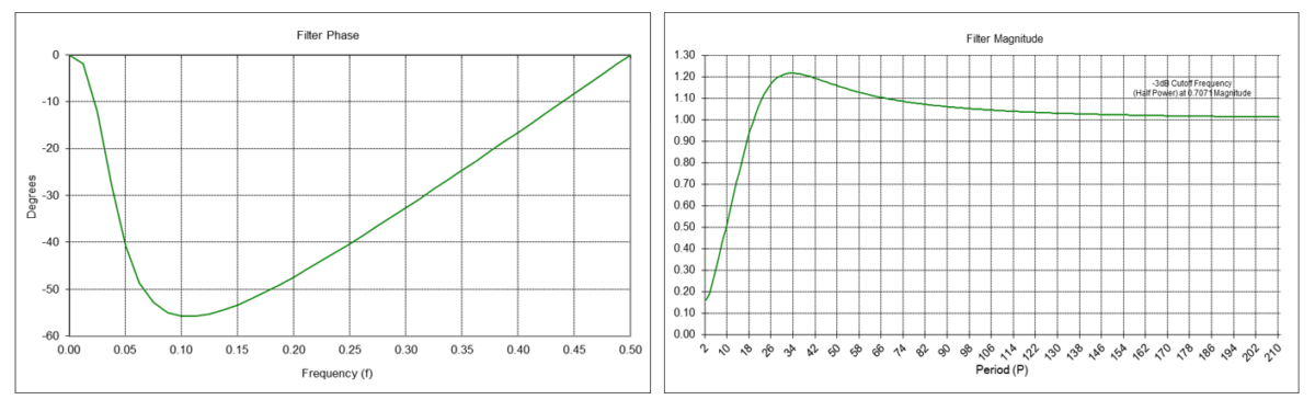
Alpha-Beta Position Tracking Filter Frequency Response (α = 0.29896, β = 0.05295)
The alpha-beta position tracking filter y0(t) is a type of IIR low pass filter, i.e., it passes frequencies below the cutoff frequency fc and attenuates frequencies above the cutoff frequency. The α and β smoothing constant values determine the cutoff frequency of the filter.
IIR position tracking filter difference equation (requires proper initialization):

Example: Alpha-beta position tracking filter using random acceleration-based smoothing constants α = 0.29896 and β = 0.05295 The filter has a -3 dB (half power) cutoff frequency fc of approximately 0.0769 (cutoff period Pc of approximately 13-time samples), similar to that of a double moving average mean filter with length N = 10. There is a magnitude peak above 1.0 (i.e., 0 dB) at a period of approximately 33-time samples.
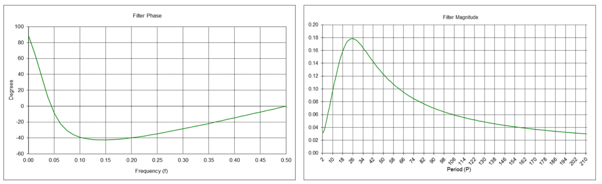
Alpha-Beta Velocity Tracking Filter Frequency Response (α = 0.29896, β = 0.05295)
The alpha-beta velocity tracking filter y1(t) is a type of IIR bandpass filter. The filter has a center (also called “resonant”) frequency f0, corresponding to a center period P0, which passes at maximum power. The α and β smoothing constant values determine the center frequency f0 of the filter.
IIR velocity tracking filter difference equation (requires proper initialization):
Example: Alpha-beta velocity tracking filter using random acceleration-based smoothing constants α = 0.29896 and β = 0.05295
The center frequency f0 is approximately 0.04, which corresponds to a center period P0 of approximately 25 time samples, similar to that of a double moving average linear trend filter with length N = 10.

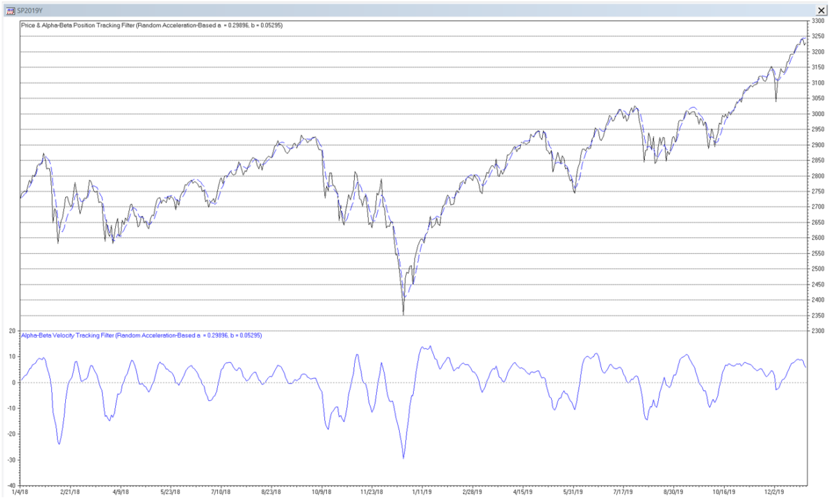
Random Acceleration-Based Alpha-Beta Position and Velocity Tracking Filter Example
The following S&P 500 daily price chart shows the alpha-beta position (dashed blue line) and velocity (solid blue line) tracking filter using random acceleration-based smoothing constants α = 0.29896 and β = 0.05295.
Trading signals using alpha-beta position and velocity tracking filters can potentially be generated in a similar manner to those described for double moving average mean and linear trend filters.
7. Prediction and Prediction Accuracy
For a time series with an underlying second order process, assuming that the current linear trend (velocity) y1(t) is locally constant and using the same time step convention as is used for the one time-step predictions above, mean (position) predictions y0^ at future integer time steps can be made at time step t, using the following equation:

One measure that can be used to evaluate the appropriate filter length or smoothing constant values to use with a particular time series is to calculate the root mean square error (RMSE) of the one time-step predictions of the filter over a sample of observations. The one time-step prediction error xe(t) at each time step t is the difference between the input value x(t) at time step t and the prediction y0^(t-1) made for time step t at the previous time step t-1:
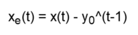
The root mean square error over a sample of N observations is:
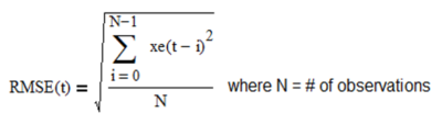
In general, the filter length or smoothing constant values that produce the minimum RMSE can be helpful in determining a useful setting. Unlike filters that are modeled on first order processes, filters modeled on second order processes will usually have a non-trivial minimum RMSE value when applied to financial time series. However, values that minimize RMSE may not necessarily correspond to maximum trading profitability. In addition, the value that minimizes RMSE in one sample of observations will not necessarily be the same in a different sample, due to the volatility, non-normality, and non-stationarity usually observed in financial time series.
8. General Comments on Second Order Process Filters
While mean (position) filters modeled on second-order processes are able to follow input time series that contain a locally constant linear trend (velocity) with less lag compared to filters modeled on first-order processes, if the input time series contains a non-linear trend (acceleration or higher-order maneuver), for example, second-order mean (position) filter estimates will lag the input.
Second-order process linear trend (velocity) filters are bandpass filters that are “tuned” to a specific center frequency or period, based on the filter coefficients, with an associated phase response. As a result, if the input time series contains a cycle with a period that is less than the center period of the filter, the filter output will crest (trough) after the input time series cycle crest (trough). Conversely, if the input time series cycle period is greater than the center period, the filter output will crest (trough) before the input time series crest (trough). This behavior can be observed in the linear trend (velocity) filter outputs in the S&P 500 daily price charts.
Since financial time series are non-stationary with means and variances that change over time, the use of filters with fixed parameters will not perform well at all times for trading purposes. As a result, filter coefficients that are “fitted” to a particular portion of a time series history will not necessarily produce good results in the future.
Acknowledgments
I would like to thank Larry Stabile for reviewing this article and providing many helpful comments and suggestions.
Appendix 1 – Double Moving Average Equations Derivation
For a second order process input with mean a, linear trend b, and normally distributed random noise ε(t):
a single moving average of length N estimates the mean value at each time step t over the last N observations. Assuming for a moment that ε(t) = 0, the mean estimates MA1(t) form a straight-line ramp with slope b and lag (N – 1)/2 relative to x(t):
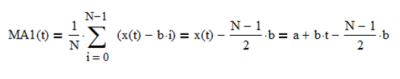
A single moving average MA2(t), also of length N, of the mean estimates MA1(t) forms a straight-line ramp with slope b and lag (N – 1)/2 parallel to MA1(t):
Letting the mean filter output y0(t) = a + b*t and the linear trend filter output y1(t) = b:
and solving the two equations for mean y0(t) and linear trend y1(t) gives:
Appendix 2 – Double Linear Weighted Moving Average Equations Derivation
For a second order process input with mean a, linear trend b, and normally distributed random noise ε(t):
a single linear weighted moving average of length N estimates the mean value at each time step t over the last N observations. Assuming for a moment that ε(t) = 0, the mean estimates LWMA1(t) form a straight-line ramp with slope b and lag (N – 1)/3 relative to x(t):
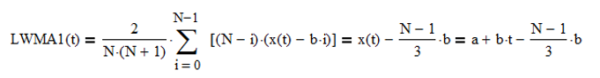
A single linear weighted moving average LWMA2(t), also of length N, of the mean estimates LWMA1(t) forms a straight-line ramp with slope b and lag (N – 1)/3 parallel to LWMA1(t):
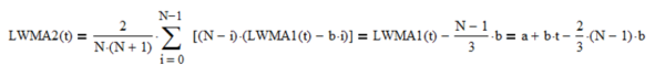
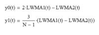
Letting the mean filter output y0(t) = a + b*t and the linear trend filter output y1(t) = b:
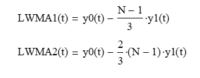
and solving the two equations for mean y0(t) and linear trend y1(t) gives:
Appendix 3 – Double Exponential Smoothing Equations Derivation
For a second order process input with mean a, linear trend b, and normally distributed random noise ε(t):
single exponential smoothing with smoothing constant α estimates the mean value at each time step t. Assuming for a moment that ε(t) = 0, the mean estimates ES1(t) form a straight-line ramp with slope b and lag (1 – α)/α (with an initial transient (1- α)t that goes to zero as t increases) relative to x(t):
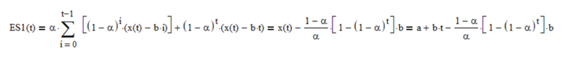
Single exponential smoothing ES2(t), also with smoothing constant α, of the mean estimates ES1(t) forms a straight-line ramp with slope b and lag (1 – α)/α (with an initial transient (1- α)t that goes to zero as t increases) parallel to ES1(t):

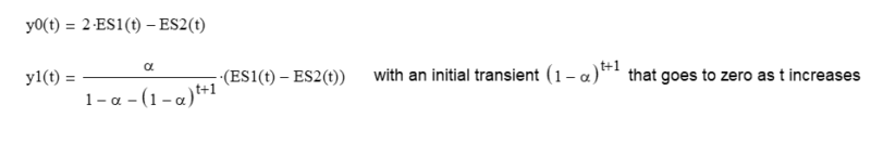
Letting the mean filter output y0(t) = a + b*t and the linear trend filter output y1(t) = b:
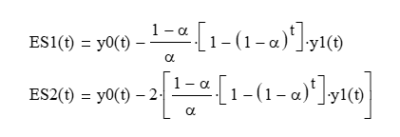
and solving the two equations for mean y0(t) and linear trend y1(t) gives:
References[+]
| ↑1 | See this post for further background on the discussion below and see here for some details on simple trend-following systems |
|---|---|
| ↑2 | Brown, R. G., Smoothing, Forecasting, and Prediction of Discrete Time Series, Prentice Hall, 1962 |
| ↑3 | Brown, R. G., Smoothing, Forecasting, and Prediction of Discrete Time Series, Prentice Hall, 1962 |
| ↑4 | Benedict, T. R., and Bordner, G. W., “Synthesis of an Optimal Set of Radar Track-While-Scan Smoothing Equations”, IRE Transactions on Automatic Control, AC-7 (4), 27-32, July 1962. |
| ↑5 | Navarro, A. M., “General Properties of Alpha Beta and Alpha Beta Gamma Tracking Filters”, Report PHL 1977-02, Physics Laboratory, National Defense Research Organization, Netherlands, January 1977. |
| ↑6 | Kalata, P. R., “The Tracking Index: A Generalized Parameter for α-β and α-β-γ Target Trackers”, IEEE Transactions on Aerospace and Electronic Systems, AES-20 (2), 174-182, March 1984. |
| ↑7 | Painter, J. H., Kerstetter, D., and Jowers, S., “Reconciling Steady-State Kalman and Alpha-Beta Filter Design”, IEEE Transactions on Aerospace and Electronic Systems, AES-26 (6), 986-990, November 1990. |
About the Author: Henry Stern
—
Important Disclosures
For informational and educational purposes only and should not be construed as specific investment, accounting, legal, or tax advice. Certain information is deemed to be reliable, but its accuracy and completeness cannot be guaranteed. Third party information may become outdated or otherwise superseded without notice. Neither the Securities and Exchange Commission (SEC) nor any other federal or state agency has approved, determined the accuracy, or confirmed the adequacy of this article.
The views and opinions expressed herein are those of the author and do not necessarily reflect the views of Alpha Architect, its affiliates or its employees. Our full disclosures are available here. Definitions of common statistics used in our analysis are available here (towards the bottom).
Join thousands of other readers and subscribe to our blog.