Original: October, 2023
Updated: March, 2025
1. Introduction
Financial time series that are structured as data sampled at a uniform time interval, e.g., hourly, daily, weekly, or monthly, are called discrete-time time series and referred to, from a digital signal processing (DSP) perspective, as being in the “time domain.” Technical market analysts generally study financial time series in the time domain. For example, a price chart displays time series values at each discrete time sample observation.
Since financial time series data are digital by nature, various digital filtering-based indicators, such as moving averages and time series momentum, are used by analysts to transform and analyze them, e.g., to identify trading opportunities presented by trends. Given that financial time series, by their nature, are challenging to analyze due to non-stationarity, volatility, noise, and other factors, analysts are interested in the ability of such indicators to rapidly respond to changes in trend direction while also minimizing noise that can result in “whipsaw” trading losses.
This article examines four digital filters commonly used for trend-following:
- moving average
- linear weighted moving average
- exponential smoothing
- time series momentum
from a time domain perspective, employing several time response specifications, including ones used in control system engineering [1]:
- delay time
- rise time
- lag
- steady-state error
- trend reversal time.
These specifications are compared to the filter variance reduction ratio, a measure of noise rejection, to illustrate the inherent trade-off between filter responsiveness and noise minimization.
Note that time series can also be analyzed in the DSP “frequency domain,” where they are considered as being composed of sinusoidal functions or frequency components, each of which has a specific amplitude (a measure of maximum displacement from equilibrium) and phase (a measure of angular shift). Previous articles in this series have analyzed financial time series and various technical indicators in the frequency domain. For example, see [2], which examines the frequency domain characteristics of the four filters and several others. It also contains a review of DSP-related terminology and topics, such as finite impulse response (FIR) filters, infinite impulse response (IIR) filters, low pass filters, differentiators, frequency response, etc.
2. Time Domain Concepts
This section provides brief overviews of the time domain concepts used in this article. More detailed discussions of these and related concepts can be found in various textbooks, such as [3] and [4].
Unit Pulse Response
The unit pulse response of a discrete-time linear time-invariant (LTI) system, such as a digital filter, is its output as a function of time in response to a discrete-time unit pulse input. The unit pulse function is denoted by δ(t), the Kronecker delta function, where:

The unit pulse function is illustrated in the following graph.
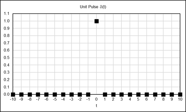
The response of a filter to a unit pulse input completely defines the filter, i.e., both its time domain and frequency domain responses, since the unit pulse contains all frequencies. In the time domain, the filter response to a unit pulse input is represented by its unit pulse response coefficients h(i), where each h(i) coefficient denotes the filter response to the time-shifted unit pulse δ(t-i). For both finite impulse response (FIR) and infinite impulse response (IIR) filters, the unit pulse response coefficients h(i) are used as the basis for calculating the time domain specifications, as explained in Section 4.
Unit Step Response
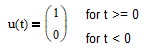
The unit step response of a discrete-time LTI system or filter is its output as a function of time in response to a discrete-time unit step input. The unit step function is denoted by u(t) where:
The unit step function is illustrated in the following graph.
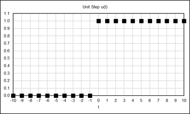
For example, the unit step is used to model an abrupt change in the input, such as when a voltage is applied to a circuit by turning on a switch. Security prices are also subject to sudden jumps and drops in response to economic and political events, company and industry news, earnings reports, etc. The unit step responses of the filters are used to measure delay time and rise time, as explained in Section 4.
Unit Ramp Response
The unit ramp response of a discrete-time LTI system or filter is its output as a function of time in response to a discrete-time unit ramp input. The unit ramp function is denoted by r(t) where:
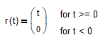
The unit ramp function is illustrated in the following graph.
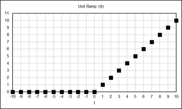
The unit ramp represents a linear trend with a slope of +1. The unit ramp response of a filter is associated with lag and steady-state error, as explained in Section 4.
Trend Reversal Response
In this article, the trend reversal response of a LTI system or filter is determined using its output as a function of time in response to a discrete-time input in the shape of an isosceles triangle, with the left edge having a slope of +1 (a positive unit ramp) and the right edge having a slope of -1 (a negative unit ramp). The trend reversal function represents an Idealized change in trend direction and is denoted by tr(t) where:
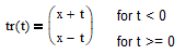
and x is the trend reversal point value at integer time t = 0. The following graph illustrates an example where x = 10.
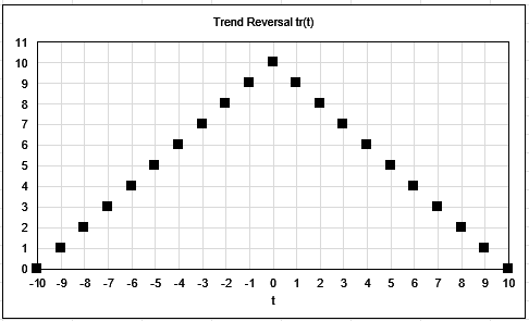
The trend reversal responses of the filters are used to calculate trend reversal time, as explained in Section 4.
3. Overview of the Filters
This section provides brief overviews of the four filters analyzed in this article. For additional details, see [2].
Moving Average (MA)
Moving average (MA) is a FIR low pass filter where the filter coefficients have equal values. Low pass filters pass low frequencies (long periods) and attenuate high frequencies (short periods) in the input signal and are commonly used to reduce noise, since noise is associated with high frequencies. The equation of a MA filter with a length of N integer time samples is:
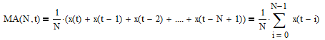
where x(t-i) is the filter input, e.g., prices, at integer time t-i. A commonly-used trading signal is generated when the current price crosses above (buy) or below (sell) the moving average.
Linear Weighted Moving Average (LWMA)
Linear weighted moving average (LWMA) is a FIR low pass filter where the filter coefficients are linearly weighted with the greatest weights placed on the most recent input values. The equation of a LWMA filter with a length of M integer time samples is:

Similar to the MA filter, a commonly-used trading signal is generated when the current price crosses above (buy) or below (sell) the linear weighted moving average.
Exponential Smoothing (ES)
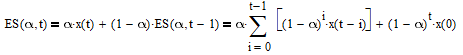
Exponential smoothing (ES) is an IIR low pass filter where a smoothing constant α is applied to the current input value and (1 – α) is applied to the previous filter output value. The equation of an ES filter with smoothing constant α is:
where 0 <= α <= 1. Similar to the MA and LWMA filters, a commonly-used trading signal is generated when the current price crosses above (buy) or below (sell) the exponential smoothing.
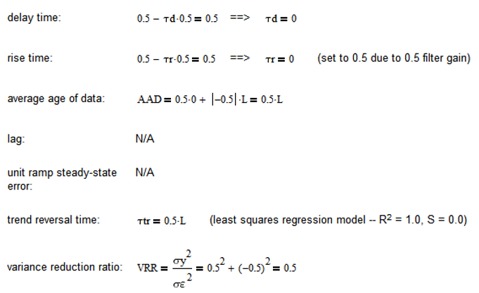
Time Series Momentum (TSMOM)
Time series momentum (TSMOM) is a FIR differentiator which calculates the difference between two samples of an input signal that are separated in time by a lookback, a fixed number of time samples. The output of a differentiator is proportional to the rate of change, i.e., the derivative with respect to time, of the input, so differentiators are commonly used to detect changes in trend. The TSMOM equation with a lookback of L integer time samples is:
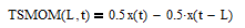
TSMOM is the simplest FIR differentiator, since it only uses two input time samples. The filter gain is often set to 1.0 but is set here to 0.5 so that the maximum magnitude frequency response of the filter is 1.0 (0 dB). A commonly-used trading signal is generated when TSMOM output changes sign, i.e., crosses above (buy) or below (sell) zero.
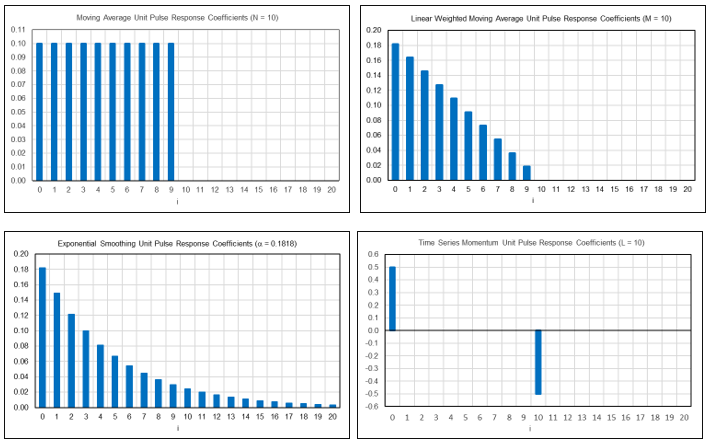
Example Filter Unit Pulse Response Coefficients
The graphs below show representative examples of the unit pulse response coefficients of the four filters, using the indicated parameter values, i.e., moving average length N = 10, linear weighted moving average length M = 10, exponential smoothing constant α = 0.1818, and TSMOM lookback L = 10, with the exponential smoothing coefficients displayed limited to the first 21.
4. Filter Time Domain Specifications
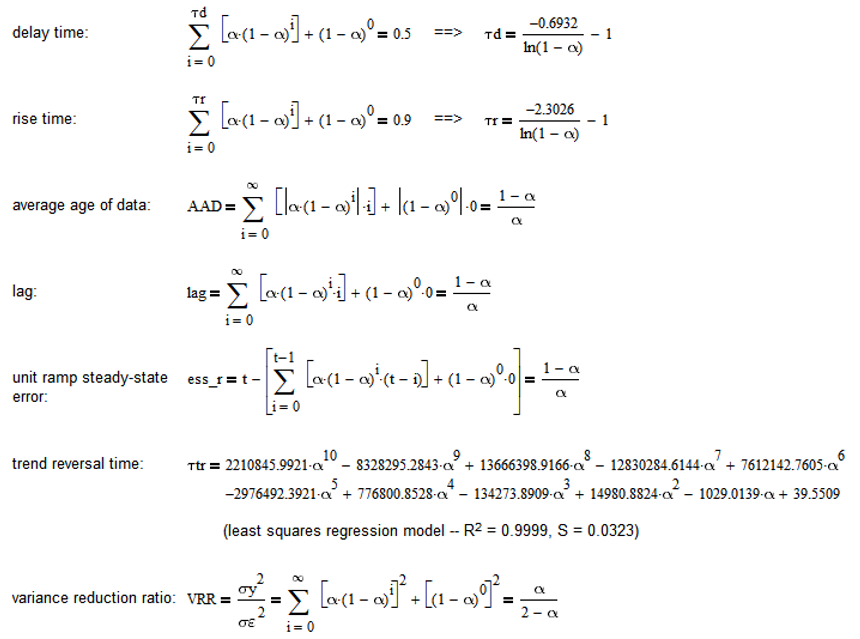
This section details the filter time domain specifications analyzed in this article. The specifications are calculated using the unit pulse response coefficients h(i) of the filters. The specification equations of the filters can be found in the appendices.
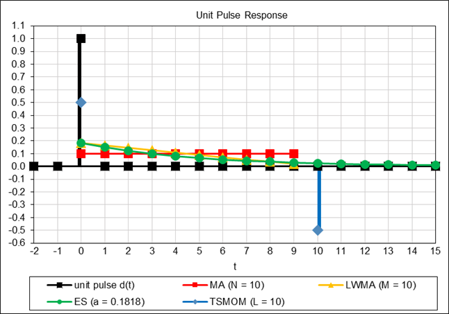
The graph below shows the unit pulse responses of the four filters, using the example filter parameter values. (Note: The square markers in the following response and specification graphs indicate the discrete values at each integer time t. The connecting lines have been added for visual enhancement and do not represent continuous values.)
Delay Time
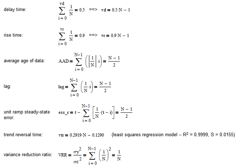
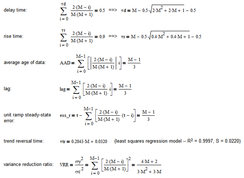
Delay time τd is measured as the number of time steps, starting at t = 0, that is required for the filter output to rise from 0% to 50% (0.5) of its final value in response to a unit step input. Delay time can be calculated using the following equation:

and solving for τd.
The graph below illustrates the delay times of the four filters, using the example filter parameter values. The delay time is observed when the filter output reaches the 0.5 level.
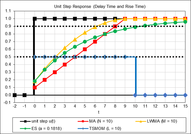
Rise Time
Rise time τr is measured in this article as the number of time steps required for the filter output to rise from 0% to 90% (0.9) of its final value in response to a unit step input. On this basis, rise time can be calculated using the following equation:

and solving for τr.
Note that different starting and ending percentages can be selected to measure rise time, depending on the type of filter and other considerations. In the case of TSMOM, which is a differentiator, rise time is measured as the number of time steps required for the filter output to rise from 0 to the 0.5 level, since the filter gain is 0.5. In this case, the rise time equation is:

The graph above also illustrates the rise times of the four filters, using the example filter parameter values. In the case of TSMOM, the delay and rise times are both the same, i.e., zero.
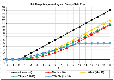
Lag
As explained in [2]. MA, LWMA, and ES are low pass filters that are modeled on the assumption that the underlying process of the input has a locally constant mean value and does not contain trends. These filters are designed to estimate the mean value of the input and not to estimate trends. As a result, the output of a first order low pass filter will exhibit lag, or a time delay, relative to the filter input if the input contains a trend.
Lag can be generally calculated as the sum of the time-weighted filter unit pulse response coefficients h(i) [5]:
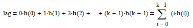
where k = number of filter unit pulse response coefficients and h(i) = unit pulse response coefficient for i = 0, 1, 2, …, k-1. Note that the time weights are the same as the unit ramp. As a result, lag is typically measured by the response of a filter to a unit ramp input once the filter output has reached a steady-state condition, which begins at the point when the ramp input has reached all of the filter coefficients. Prior to reaching steady-state, the filter response is said to be in a transient state as it adjusts over time to the change in the input. Steady-state occurs after all transient effects have subsided.
The graph below illustrates the lags of the three low pass filters, using the example filter parameter values. For the two FIR low pass filters MA and LWMA, steady-state lag begins at time step t = N – 1 for the MA filter and t = M – 1 for the LWMA filter. Since ES is an IIR low pass filter with an infinite transient response, steady-state can be considered to occur at approximately 99% rise time, which is at time step t = (-4.6052/ln(1 – α)) – 1 where ln is the natural logarithm. The graph also includes TSMOM, a differentiator, where the filter output reaches steady-state at time step t = L. The lag specification is not applicable to differentiators and other non-low pass filters. Note that using a ramp input with a slope other than +1 results in the same relative filter responses.
The lag of low pass filters modeled on a first order process can be used as a way to “sidestep” some of the noise and short-term fluctuations during a trend or cycle but at the cost of delayed response once the trend or cycle begins or ends.
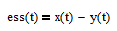
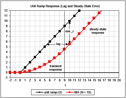
Steady-State Error
Steady-state error ess is defined as the difference between the filter input x(t) and the filter output y(t) when the filter is in a steady-state condition:
For low pass filters modeled on a first order process, in response to a unit ramp input, which has a slope of +1 (i.e., one unit of increase per one unit of time), the steady-state error ess_r equals the lag, as illustrated in the example graph below for a MA filter with length N = 10, where steady-state begins at time step t = 9. Note that the lag and ess_r form the sides of an isosceles right triangle.
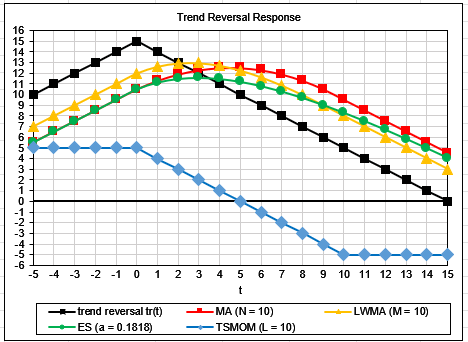
Trend Reversal Time
In the case of MA, LWMA, and ES, trend reversal time is the number of time steps, starting at t = 0, required for the filter output to intercept the unit trend reversal function input following the trend reversal point where the trend changes direction. In the case of TSMOM, trend reversal time is the number of time steps required for filter output to intercept the zero line following the trend reversal point.
The following graph illustrates the trend reversal times of the four filters, using the example filter parameter values. Note that using a trend reversal input with slopes other than +1 and -1 results in the same relative filter responses.
The equations used to estimate the trend reversal times of the filters that appear in the appendices were determined by applying least squares regression to a series of measurements of the intercept or zero-line crossing times of each filter across a range of filter parameter values. All of the regression models have coefficients of determination R2 very close to 1 and small standard errors of estimate S, as shown in the appendices.
As a side note, as demonstrated in [2], a TSMOM filter with lookback L changes sign at the same time as a MA filter with length N passes an inflection point, i.e., the MA changes direction, when L = N. This mathematical relationship can be observed in the graph above, where the TSMOM with L = 10 crosses below the zero line at the same time as the MA with N = 10 changes direction and starts to decrease, both occurring at time step t = 6 in this example.
Additional discussion regarding filter trend reversal response can be found in [6].
Variance Reduction Ratio
For time series containing normally distributed random noise ε(t) ~ N(0, σε2), the variance reduction ratio (VRR) of a filter measures the reduction in the variance of the filter output y(t) relative to the variance of the filter input and is calculated by summing the squares of the filter unit pulse response coefficients h(i) [5]. VRR is the ratio of the filter output variance to the input variance:
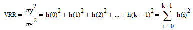
where k = number of filter unit pulse response coefficients and h(i) = unit pulse response coefficient for i = 0, 1, 2, …, k-1. Note that this calculation is equivalent to the Herfindahl-Hirschman Index [6]. The smaller the ratio, the greater the noise reduction. For example, VRR = 0 indicates complete noise reduction, whereas VRR = 1 indicates no noise reduction.
5. Filter Specification Comparison
The following graphs show the specifications of the four filters across a range of filter parameter values. As mentioned previously, the specification equations of the filters can be found in the appendices.
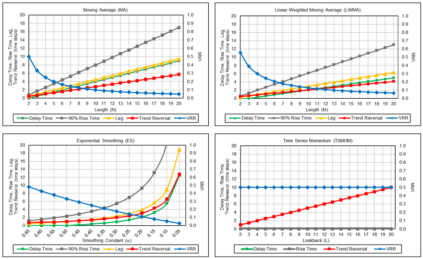
For the three low pass filters, the graphs indicate that the larger the filter lengths N or M or the smaller the smoothing constant α, the smaller the VRR but also the greater the delay time, rise time, lag, and trend reversal time. For TSMOM, a differentiator, trend reversal time increases with increasing L, whereas delay time and rise time (both zero) and also VRR remain constant.
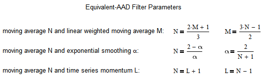
Filters with Equivalent Average Age of Data
In order for the filter specifications to be comparable, the filter parameter values need to be standardized. Since average age of data (AAD) is commonly used in the technical analysis literature when calculating equivalent filter parameters (see [2] for details concerning the AAD calculation), the method chosen here is to convert the filter parameters to the corresponding moving average lengths so they have equivalent AAD, i.e., equivalent average age of the data passing through them. The filter parameter conversion equations are shown below.
The graphs below show the filter specifications standardized on their equivalent-AAD MA filter lengths.
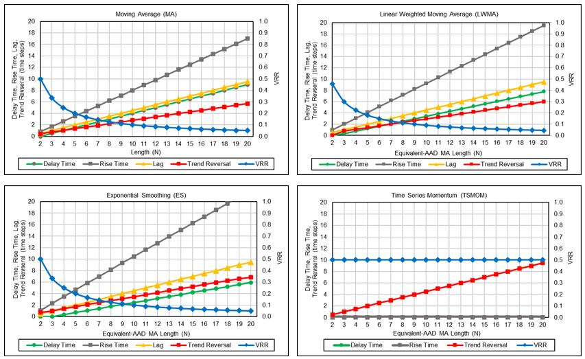
The graphs indicate that:
- On an equivalent-AAD basis, the three low pass filters have approximately equal lags and, consequently, equal steady-state errors.
- On an equivalent-AAD basis, the three low pass filters have approximately equal VRRs, with the LWMA VRR being slightly lower than the others. TSMOM, a differentiator, has the highest VRR, i.e., the least noise reduction, of all the filters.
- With respect to the trade-off with VRR, among the three low pass filters, ES has the shortest delay time and MA has the shortest rise time and trend reversal time. On the other hand, MA has the longest delay time and ES has the longest rise time and trend reversal time.
- TSMOM has the shortest delay time and rise time (both zero) of all the filters, but it also has the longest trend reversal time.
Acknowledgements
I would like to thank Valeriy Zakamulin and Larry Stabile for reviewing this article and providing many helpful comments and suggestions.
Appendix 1 – Moving Average (MA) Filter Specifications
Appendix 2 – Linear Weighted Moving Average (LWMA) Filter Specifications
Appendix 3 – Exponential Smoothing (ES) Filter Specifications
Appendix 4 – Time Series Momentum (TSMOM) Filter Specifications
References
[1] Gowda, K., “Control Systems 2.4 – Time Response Specifications”, March 2021; available online at https://www.circuitbread.com/tutorials/time-response-specifications-2.4.
[2] Stern, H., “An Introduction to Digital Signal Processing for Trend Following”, August, 2020, updated: March, 2025; available online at https://alphaarchitect.com/2020/08/an-introduction-to-digital-signal-processing-for-trend-following/.
[3] Schwarz, R. J. and Friedland, B., Linear Systems, McGraw-Hill, 1965.
[4] Oppenheim, A. V., Willsky, A. S., and Young, I. T., Signals and Systems, Prentice Hall, 1983.
[5] Brown, R. G., Smoothing, Forecasting, and Prediction of Discrete Time Series, Prentice Hall, 1962.
[6] Zakamulin, V., Market Timing with Moving Averages: The Anatomy and Performance of Trading Rules, Springer, 2017.
About the Author: Henry Stern
—
Important Disclosures
For informational and educational purposes only and should not be construed as specific investment, accounting, legal, or tax advice. Certain information is deemed to be reliable, but its accuracy and completeness cannot be guaranteed. Third party information may become outdated or otherwise superseded without notice. Neither the Securities and Exchange Commission (SEC) nor any other federal or state agency has approved, determined the accuracy, or confirmed the adequacy of this article.
The views and opinions expressed herein are those of the author and do not necessarily reflect the views of Alpha Architect, its affiliates or its employees. Our full disclosures are available here. Definitions of common statistics used in our analysis are available here (towards the bottom).
Join thousands of other readers and subscribe to our blog.