Factor investing research has a long storied past. Fama and French’s 1992 and 1993 papers arguably put factor investing “on the map,” but truth be told, factor investing is an old topic with roots grounded in the so-called arbitrage pricing theory. We have a longer piece on the history of factor investing here.
There is a monster empirical research effort to determine which factors describe stock returns in the historical data (many consider this a data-mining effort). A criticism of the “let’s see what the data says” approach is that these empirical models often lack a clear economic foundation or theory. In other words, if sunspots predict stock returns in the data, we should not claim victory. Or for a more realistic example, instead of focusing on SMB (size) and HML (value) because they “work,” we should focus on using SMB and HML in our factor models because they are tied to economic theories that are grounded on first principles. Many people have gone this direction, but the theoretical models they’ve developed, while sensible, do a terrible job describing reality (e.g., CAPM).
Bottom line: factor models that describe the movement of expected stock returns should be tied to economic foundations AND they should do a reasonable job explaining the patterns in historical data. This combination helps alleviate data-mining concerns. Simple in theory, but building a reasonable theory and having it roughly match historical data is quite difficult!
Lu Zhang and his colleagues have put in a good faith effort to build factor models that are backed by economic models and do a great job describing historical stock return patterns. One can argue that their theory is wrong, but at least they are generating a theory that motivates their factor model. And because we believe Lu Zhange et al. are arguably on the cutting edge of factor investing research, we’ve focused on covering their research (here, here, and here) and interviewing Lu to get his insights.
The piece that follows related to their latest research papers, “Which Factors” and “q5.“
Two New Papers: Which Factors and q5
Wes: Lu, you and your colleagues have been busy. Really busy. Since we covered your last research paper, “Replicating Anomalies,” which was a monster research effort already, you and your team have managed to grind out two new papers: “Which Factors” and “q5.” Where do you get the time?
Lu: We have a very efficient team. Kewei Hou, Chen Xue, and I have been working closely together since 2011. Our q-factor paper is the most cited article published at Review of Financial Studies in 2015. Our work on “Replicating Anomalies” has also been well received, in both industry and academia. Haitao Mo joined us a couple years ago. All three of my collaborators are superior empiricists. We go through internal, independent replications every time we report new results in a working paper. We model after Fama and French on the quality of empirical execution. We feel comfortable with our intellectual product.
Wes: Walk us through the key differences between the two new papers.
Lu: We have just circulated the updated drafts for both papers, now dated July 2018. Check them out on my research page or SSRN page. The title for “Motivating Factors” has changed to “Which Factors?” to reflect the content of its revised draft. The two papers are complementary.
The key message for “q5” is to augment the q-factor model with a new expected growth factor to form the q5 model. Using the vast set of 158 significant anomalies from “Replicating Anomalies” as testing deciles in a large-scale empirical horse race, we show (i) the q5 model is the best performing model; and (ii) the q-factor model already compares well with the Fama-French 6-factor model and other models.
The focus of “Which Factors?” is on spanning regressions and on the conceptual foundation of factor models. We reproduce and replicate the Stambaugh-Yuan (2017) 4-factor model and the Daniel-Hirshleifer-Sun (2018) 3-factor model. Reproduction means we follow their exact procedures, and replication means we follow the standard approach per Fama and French (1993). We find that the Stambaugh-Yuan and Daniel-Hirshleifer-Sun models are both sensitive to their construction. Using the standard approach, which ensures that we compare apples with apples, weakens their performance, often substantially.
Conceptually, the paper on “Which Factors?” raises some concerns on motivating the Fama-French 5-factor model from valuation theory. In particular, consistent with the investment CAPM, valuation theory also implies a positive relationship between the expected investment and the 1-period-ahead expected return. As such, CMA can only be motivated from the market-to-book term in the valuation equation via the economic linkage between investment and value, which is, in turn, a key insight from the investment CAPM.
Digging into the “q5” paper
Wes: Let’s start with q5. I got to ask a non-quant question first – what’s with the funky name and the superscript character? Any backstory on that?
Lu: The funky name is Kewei’s idea. We played with “Q5” for a while like the Audi SUV, which I used to drive. But “q5” seems cool. I like its nerdy feel.
Wes: Okay, digging back into the details. Tell us a little more about your expected growth factor. How’s it measured?
Lu: We measure the expected investment growth as the fitted component from monthly cross-sectional regressions of the 1-year-ahead investment-to-assets change on the log of Tobin’s q, operating cash flows, and the change in return on equity in the prior 120-month rolling window. Then we construct the expected growth factor from monthly, independent 2-by-3 sorts on size and the expected growth.
Wes: Is there any way to make a simple version of the measure that doesn’t require a rolling regression estimate? For example, for the forecasted investment growth variable, could someone use recent TTM (trailing twelve months) ROE growth and be in the ballpark?
Lu: The change in return on equity is included when we forecast investment growth in the latest draft of the q5 paper. We include this variable to capture some of the short-term dynamics of investment growth. However, we show that the ratio of operating cash flows to book assets measured as in Ball, Gerakos, Linnainmaa, and Nikolaev (2016) has stronger predictive power for investment growth.
This result makes economic sense. The Ball et al. measure takes away accruals, but include R&D expenses. All else equal, high accruals mean low cash flows available for investments going forward, and thus low expected growth. High accruals also mean high past growth, which implies low expected growth, due to the strong mean version in growth rates. Finally, high R&D expenses mean low current return on equity, due to the standard accounting practice, but induce high expected growth going forward. In fact, cash flows also take care of (to some extent) the accounting problem for other intangible investments such as advertising, employee training, information technology, organizational capital, etc.
Wes: You mention that firms with high expected investment growth should earn higher expected returns. Can you elaborate?
Lu: Sure. The intuition is analogous to (but a bit more involved than) that behind the positive relation between profitability and the expected return in our q-factor paper.
With only two periods, the investment CAPM implies that the discount rate equals the expected profitability divided by the marginal cost of investment (which rises with current investment). As such, high profitability relative to low current investment means a high discount rate, which offsets the high expected marginal benefit of current investment (expected profitability) to keep the current investment low.
In a multiperiod framework, the expected marginal benefit of current investment also increases with the expected next period investment. At the end of the next period, a firm is left with the capital generated from current investment, net of depreciation. The market value of that leftover capital is the present value of all future cash flows that it can generate (what economists call marginal q). The presence of that capital saves the firm the exact amount that equals the marginal cost of next period investment (which, again, increases with next period investment). In all, high next period investment relative to low current investment (high investment growth) means a high discount rate, which counteracts the high expected marginal benefit of current investment (the part from the expected next period investment) to keep the current investment low.
Hope the intuition is penetrable. The math equation is very clear. Words can be ambiguous.
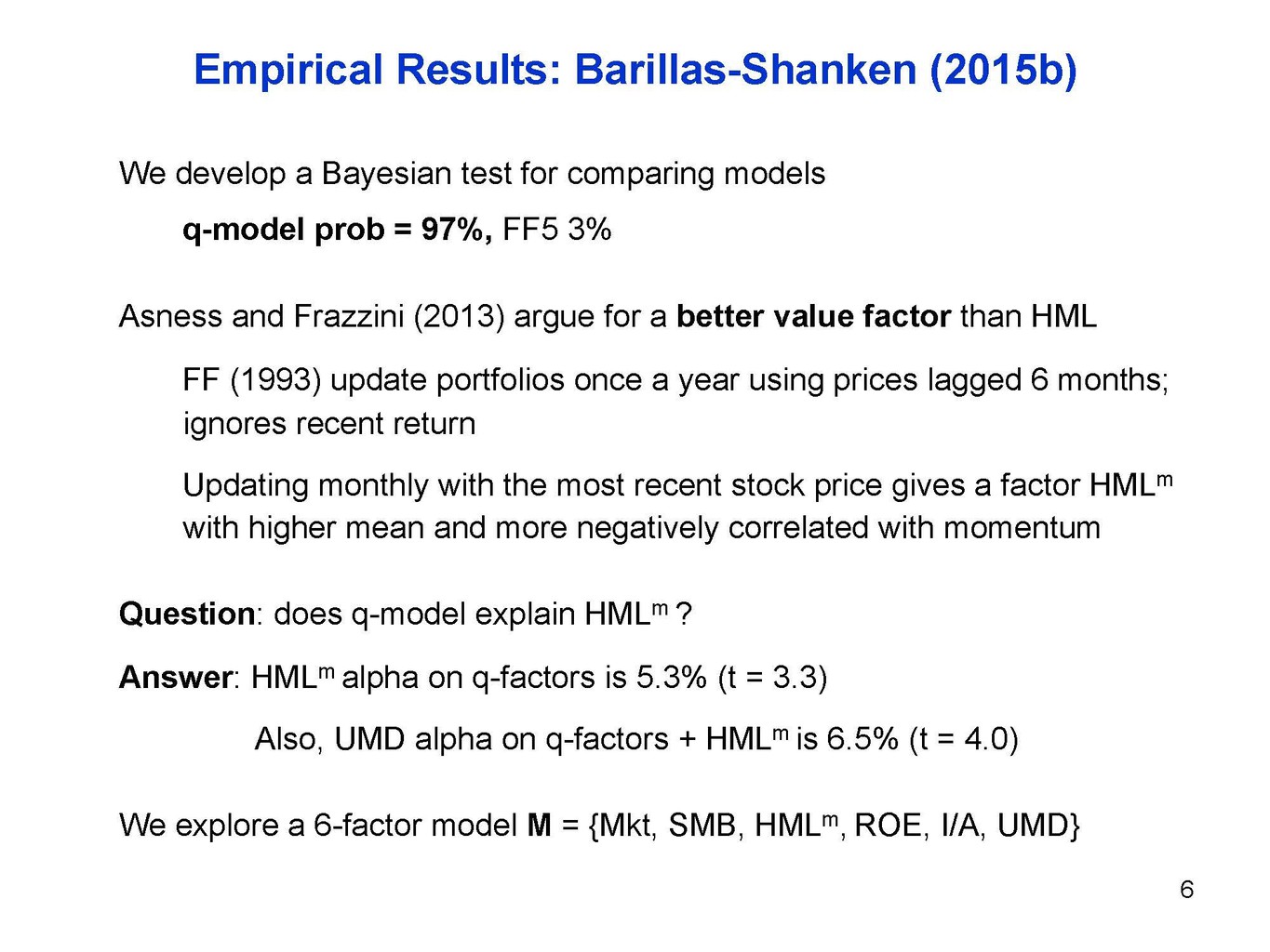
Wes: Barillas and Shanken try and identify the “best” factor model via a Bayesian lens. They find that the 6-factor model of Mkt, SMB, ROE, IA, HMLm, and UMD works the best. In other words, value and momentum are not redundant. The Fama French 5 Factor model gets demolished, and while your HXZ 4-factor model does better, their 6-factor version does better. How do you address this research?
Lu: Sure. First, the Barillas-Shanken model is purely statistical, with little economic foundation. Our q and q5 models stand out in the factors debate in that our models are the only ones with close ties to first principles in economic theory. The anomalies/factors literature is heavy-duty empirical, but we show there is a lot of economics as well.
Second, Barillas and Shanken end up picking our investment and Roe factors over Fama and French’s CMA and RMW. In fact, the truth is even stronger. Figure 1 reports page 6 in Jay Shanken’s discussion slides on our working paper on “A Comparison of New Factor Models,” from which our paper “Which Factors?” descends, in the 2015 Arizona State University Sonoran Winter Finance Conference. Shanken said in the conference that in his work in progress (at the time) with Barillas, they assigned a 50-50 diffuse prior to the q-factor model and the Fama-French 5-factor model, but found that the posterior probability of the q-factor model being true is 97%, and that of the 5-factor model is only 3%. I was happy to learn about the evidence and was hoping that Shanken’s credibility could give us a boost. However, when their working paper started to circulate in May 2015, I could not find the 97% vs. 3% evidence reported anywhere. I pointed out to Shanken, when he gave a seminar at Ohio State in November 2015, that this evidence should be reported, especially in a paper titled “Comparing Asset Pricing Models.” Still, this evidence is nowhere to be found in their published papers in 2017 Review of Financial Studies or 2018 Journal of Finance.
Figure 1. Slide 6 in Jay Shanken’s Discussion on “A Comparison of New Factor Models” at the 2015 ASU Winter Finance Conference
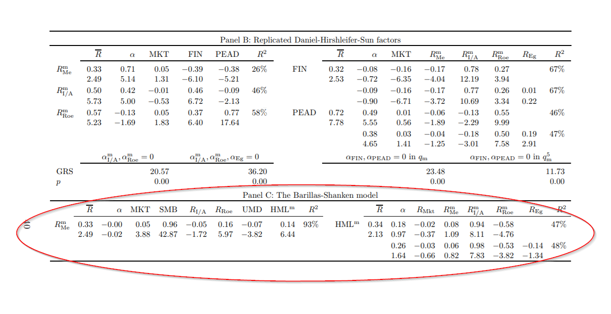
 Finally, the Barillas-Shanken tests are performed with only 11 factors, and they even argue that testing portfolios are irrelevant. This is not what we see in our tests. Using the set of 158 significant anomalies, by far the largest among the papers on competing factor models, we show in the q5 paper that the Barillas-Shanken 6-factor model does not perform well. In particular, HMLm and UMD are strongly negatively correlated, pushing up the UMD loadings in factor regressions of annually sorted value-minus-growth anomaly returns. In contrast, this empirical difficulty is entirely absent from the Fama-French 5-factor model and the q-factor model.Wes: So your expected investment growth factor seems to capture the higher frequency HML factor and the momentum factor? Can you explain the intuition behind that? What are the practical implications?
Lu: Not exactly. The Roe factor in the q-factor model already subsumes UMD, see Table 1 in “Which Factors?” which we first circulated back in September 2014. Momentum has never been a problem for us. Table 1 in “Which Factors?” shows that from January 1967 to December 2016, UMD earns on average 0.65% per month (t=3.61), but its q-factor alpha is only 0.12% (t=0.5).
However, neither the q-factor model nor the q5 model can explain Cliff’s monthly formed HML factor, HMLm. Table 4 in “Which Factors?” duly reports this evidence. However, Cliff’s insight on using more up-to-date information in monthly sorts can also be applied to the q-factor model, in which the size and investment sorts are annual, and only the Roe sort is monthly. Nothing in the investment theory says that we cannot use monthly sorts on size and investment. Once we reconstruct the q-factors with monthly sorts on size, investment, and Roe, we find that the q-factor model and the q5 model both explain HMLm. Panel C of Table 7 in “Which Factors?” reports this evidence.
Wes: What are the practical implications of this finding? How could an investor use this research to form smarter investment portfolios? Let’s say I’m trying to compound my wealth at the highest rate possible – what’s my portfolio look like?
Lu: The q5 paper shows that the q5 model is the best performing model in explaining a vast set of anomalies, and the q-factor model already compares favorably with the Fama-French 6-factor model. This means that the q-factor model and the q5 model can be used to control for “risks” in the sense of common variations in practice.
In terms of compounding wealth, buy stocks with low investment, high Roe, and high expected growth (measured with high cash flows and fast improving Roe).
“Which Factors?” paper
Okay, we’ve covered a lot already. We won’t rehash a lot of territory on your q5 paper in this section, but I did have a few questions related to the “Which Factors?” paper.
Wes: You state that the Fama and French 5-factors are not tied to valuation theory. Can you explain? Also, why should practitioners care? Also, let’s talk about CMA, the investment factor used in the Fama and Fench model. Basically asset growth for all intent and purposes. You highlight that using past investment as a proxy for expected investment doesn’t work. Explain. And why should an investor care?
Lu: These two questions are closely related, so I address them together. There are at least two difficulties with motivating the Fama-French 5-factor model from valuation theory. First, valuation theory, as formulated by Fama and French (2015), is only about the internal rate of return, which is different from the 1-period-ahead expected return, both theoretically and empirically.
More important, Fama and French motivate CMA via two steps. First, they argue that the expected investment is negatively correlated to the expected return. Second, they use current investment (asset growth) as the proxy for the expected investment. We raise concerns on both steps. Reformulating valuation theory with the 1-period-ahead expected return, we show that the relation between the expected investment and the expected return is positive per the valuation equation, consistent with the investment theory. In fact, this positive relation from the investment theory motivates our expected growth factor in the q5 paper. Moreover, we document that unlike profitability, firm-level investment is not persistent at all, casting doubt on using current investment as a proxy for the expected investment. In all, in terms of theory, only the investment CAPM can give rise to the investment and profitability factors.
Why should investors care about economic theory? Well, to guard against data mining. The investment, Roe, and expected growth factors are motivated from the first principles of real investment. As long as public traded firms are maximizing their market value of equity in their capital budgeting, at least to the first order importance, we should expect the q and q5 factor premiums to persist in the long term.
For a long time, the theory has a bad rep among investment managers. The likely reason is that the consumption CAPM, which is the dominating framework in academic finance, does not work in practice. The investment CAPM is a new breed of theory, which seems to explain the data well.
Wes: This paper seems to focus on the Fama French and the Stambaugh-Yuan factor models. One of the newer “factors” out there seems to be the low volatility or beta factor. Care to comment on this vein of research?
Lu: In the latest drafts on “Which Factors?” and “q5,” we also include the Daniel-Hirshleifer-Sun 3-factor model. We show that the Stambaugh-Yuan and Daniel et al. models’ performance is sensitive to their nonstandard factor construction. In particular, Stambaugh and Yuan use the NYSE-Amex-NASDAQ breakpoints with the 20 and 80 percentiles, and the Daniel et al.’s breakpoints are likely even more extreme, especially their financing factor. In contrast, the standard approach calls for the NYSE breakpoints with the 30 and 70 percentiles.
In other words, Stambaugh and Yuan, as well as Daniel, Hirshleifer, and Sun, are comparing apples with oranges. Their testing portfolios are formed with NYSE breakpoints and value-weighted returns, following our q-factor paper. But their factors rely on stocks in the more extreme tail distributions of the underlying characteristics.
We are not exactly sure how reliable the low volatility anomaly is, see the latest draft of our “Replicating Anomalies” (dated July 2018). About the beta anomaly, we have tried the betting-against-beta factor from the AQR Web site on the q-factor model at one point. It turns out that our Roe factor largely subsumes it. In general, as shown in our “Replicating Anomalies,” fundamentals seem to be much more important than frictions in the cross-section.
Wrapping up
Wes: A final question on interpreting factor models. Shri Santosh and colleagues highlight that it may be difficult to differentiate between the success of a factor model based on neoclassical factors or something as simple as sentiment. What do you think about this line of thought?
Lu: I agree. In fact, I wrote an earlier paper titled, “The Investment Manifesto,” published in Journal of Monetary Economics in 2013, in which I have made similar points. Basically, I view factor regressions and cross-sectional regressions are two different but largely equivalent ways of summarizing correlations in the data. No causal inferences should or can be drawn on whether the empirical relations are due to risk or sentiment. In fact, I even wrote in that paper that the concept of “risk” is an outdated notion from the consumption CAPM, which ignores the supply side of asset pricing altogether. In particular, using characteristics to forecast returns is perfectly consistent with the investment CAPM, which provides the supply theory of asset pricing.
Relatedly, I do not think “sentiment” is simple at all. It is nebulous, lacking specifics. In contrast, I think the investment CAPM is very concrete. A single equation tells us to focus on investment and Roe. The expected growth is in the equation, but less specific, alas, because one has to take a stand on what instruments to use to forecast future investment growth.
Wes: Final question: Do you know if anyone maintains a taxonomy of factor models? It would be great to have a one-stop shop on some infographic that outlines all these models.
Lu: I think the q5 paper fits the bill. Our paper on “Replicating Anomalies” takes care of the left-hand side of factor regressions, and together with “Which Factors?” the q5 paper takes care of the right-hand side.
Wes: Lu, this was awesome. Thank you very much for the insight and education. Lots to think about!
About the Author: Wesley Gray, PhD
—
Important Disclosures
For informational and educational purposes only and should not be construed as specific investment, accounting, legal, or tax advice. Certain information is deemed to be reliable, but its accuracy and completeness cannot be guaranteed. Third party information may become outdated or otherwise superseded without notice. Neither the Securities and Exchange Commission (SEC) nor any other federal or state agency has approved, determined the accuracy, or confirmed the adequacy of this article.
The views and opinions expressed herein are those of the author and do not necessarily reflect the views of Alpha Architect, its affiliates or its employees. Our full disclosures are available here. Definitions of common statistics used in our analysis are available here (towards the bottom).
Join thousands of other readers and subscribe to our blog.