One of the more popular equity strategies over the past decade is low volatility investing. Simply put, this is a systematic strategy that invests in stocks with lower volatility, either measured by Beta or standard deviation.
Why?
Well, the low-beta anomaly is the fact that in the past, academics (and practitioners) have noticed that high beta stocks have underperformed expectations from asset pricing models, while low beta stocks have outperformed expectations from asset pricing models.
As such, there are numerous papers on this topic in the academic literature. On our site, we have multiple low volatility articles here, a simulation post here, and a nice post by Larry Swedroe here.
That being said, one of the more influential papers on low-beta investing is by Andrea Frazzini and Lasse Pedersen of AQR, titled “Betting Against Beta”. A link to the paper can be found here through AQR’s website. The paper is worth a read for any investor.
The high-level idea behind the “Betting Against Beta” (BAB) factor is pretty simple:(1)
- Go long low beta stocks (and use leverage to make the beta ~1).
- Go short high beta stocks (and reduce the net exposure to make the beta ~1).
However, the construction for the Betting Against Beta (BAB) factor in the paper is definitely different than other standard academic factor portfolios. Most academic factor portfolios, such as Value (HML) and Momentum (MOM or UMD) are formed by going long the top 1/3 (i.e. the “good” stocks) and shorting the bottom 1/3 (i.e. the “bad” stocks) while controlling for size.(2)
So a natural question one may have is the following–what impact does the non-standard construction of the BAB factor have?
To answer this question directly, enter Robert Novy-Marx and Mihail Velikov, with a working paper titled “Betting Against Betting Against Beta” which I discuss below.
The paper states that the non-standard formation method creates “paper” performance that cannot be realized. Page 2 of the paper gets to a summary of the findings:
BAB achieves its high Sharpe ratio, and large, highly significant alpha relative to the common factor models, by hugely overweighting micro- and nano-cap stocks. For each dollar invested in BAB, the strategy commits on average $1.05 to stocks in the bottom 1% of total market capitalization. These stocks have limited capacity and are expensive to trade. As a result, while BAB’s “paper” performance is impressive, it is not something an investor can actually realize. Accounting for transaction costs reduces BAB’s profitability by almost 60%. While it still earns significant positive returns, it earns these by tilting toward profitability and investment, exposures for which it is fairly compensated. It does not have a significant net alpha relative to the Fama and French (2015) five-factor model.
Below we will dig into the paper, highlighting a few specific sections of the paper.
Rank-Weighting vs. Standard Factor Portfolio (L/S) Construction
The paper begins by noting that the low beta anomaly is nothing new. This was documented decades ago (Black 1972).
As mentioned above, the BAB factor is formed slightly differently than standard academic factors. So how is the BAB factor formed?
It is formed using a rank-weighting scheme.(3)
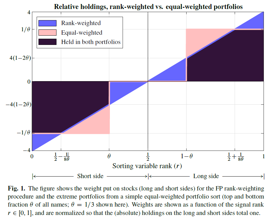
While the paper has the details, sometimes, a picture can give a clear explanation of what is going on.
Figure 1 in the paper, shown below, shows the difference between using a rank-weighted and an equal-weighted scheme.
The results are hypothetical results and are NOT an indicator of future results and do NOT represent returns that any investor actually attained. Indexes are unmanaged, do not reflect management or trading fees, and one cannot invest directly in an index. Additional information regarding the construction of these results is available upon request.
A natural question is what is the impact?
Well, using 1/3 as the cutoff amount, i.e. taking the top/bottom 1/3 on Beta for the long/short legs of the portfolio, the overlap is ~ 83%.(4)
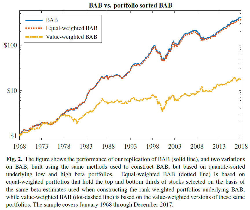
So given the high overlap (83%) between the equal-weighted BAB portfolio (taking the top & bottom 1/3) and the BAB portfolio (which uses a rank-weighted methodology), what is the impact on the performance?
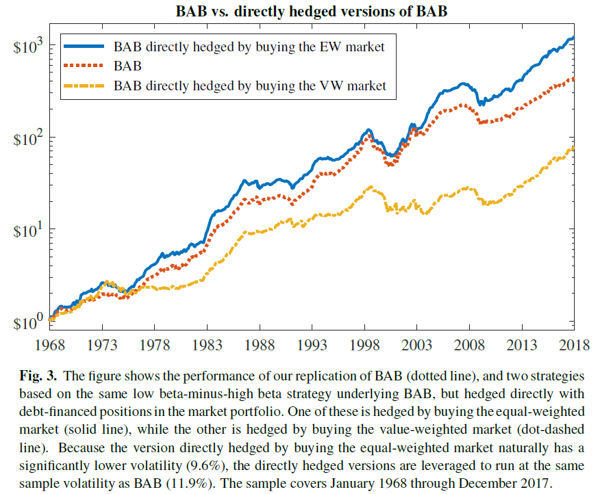
Figure 2 of the paper highlights the performance.
The results are hypothetical results and are NOT an indicator of future results and do NOT represent returns that any investor actually attained. Indexes are unmanaged, do not reflect management or trading fees, and one cannot invest directly in an index. Additional information regarding the construction of these results is available upon request.
As can be seen above, simply taking the top/bottom 1/3 based on Beta (as outlined in the original paper), and equal-weighting the portfolio (using similar leverage as the BAB factor for the long and short portfolios(5)), one generates almost the exact same result as the rank-weighting method! The correlation of the strategies is 99.6% at a monthly frequency.
In addition, figure 2 shows the performance of the value-weighted BAB portfolio, which simply takes the top/bottom 1/3 on Beta, and value-weights the positions (i.e. uses the market-cap weights). In general, this is how all the standard L/S factor portfolios are formed, such as Value (HML) and Momentum (UMD). As one can see, there is a large performance difference between the EW and VW portfolios for the non-rank-weighted BAB!
What happens to the performance of the BAB factor when value-weighted? The performance is described in the paper:
Value-weighted BAB earns significant positive excess returns over the sample, 56 bps/month with a t-statistic of 3.48, but its Sharpe ratio is less than half as large as BAB’s (0.49 compared to 1.08). It also earns most of these returns by tilting strongly to profitability and investment (loadings of 0.45 on RMW and 0.50 on CMA, with t-statistics of 6.59 and 4.86, respectively). The strategy’s alpha relative to the Fama and French five-factormodel is only 24 bps/month, and insignificant (t-statistic of 1.63).
Thus, the BAB factor, when implemented using market-cap weighting, is similar to a portfolio that loads on two other well-known factors, profitability and investment.
Section 2 of the paper (skipped here for brevity) shows that the leveraging method, which is using leverage on the low-beta portfolio to increase this exposure while reducing the net exposure on the high-beta portfolio, also embeds equal-weighted hedging in the portfolio. I recommend interested readers dig into this section of the paper, while the summary can be seen in the footnote here.(6)
The Costs of Trading BAB
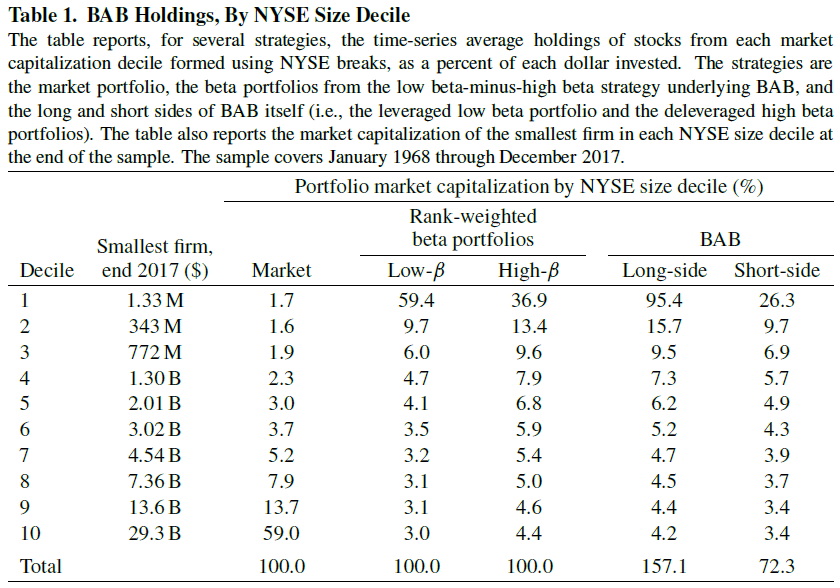
As shown above, the BAB portfolio is similar to an equal-weighted (EW) portfolio. However, sticking with the original construction, what stocks does the original BAB portfolio invest in, and is this factor tradeable?
To answer this question, we examine Table 1 in the paper, shown below. As was discussed above, the BAB factor uses leverage on the low beta portfolio to make the beta ~ 1, while reducing the exposure on the high beta portfolio to make the portfolio ~ 1. Thus, in columns 4 & 5, the total allocations sum to 100% for the long and short books. However, in columns 6 & 7, the long portfolio of BAB has 157.1% net exposure while the short portfolio has a 72.3% net exposure.
The results are hypothetical results and are NOT an indicator of future results and do NOT represent returns that any investor actually attained. Indexes are unmanaged, do not reflect management or trading fees, and one cannot invest directly in an index. Additional information regarding the construction of these results is available upon request.
As can be seen above, there is a large allocation to stocks in the bottom decile based on market-cap. Using the original BAB approach, around 110% of the long-portfolio are invested in the two smallest deciles based on market-cap! This would include firms with market caps below $772mm (as of 12/31/2017 from the table above showing the smallest firm in decile 3).
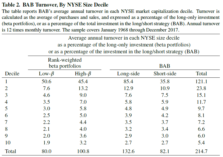
However, trading small-cap stocks, in and of itself, is only one part of trading costs. The second question is what is the turnover within the portfolios? This is shown in Table 2 below.
The results are hypothetical results and are NOT an indicator of future results and do NOT represent returns that any investor actually attained. Indexes are unmanaged, do not reflect management or trading fees, and one cannot invest directly in an index. Additional information regarding the construction of these results is available upon request.
Thus, there may be some issues with trying to trade the BAB portfolio as (1) there are many micro-cap firms in the portfolio and (2) within the micro-cap portfolio, there is high turnover.
So what happens when one accounts for trading costs?
Figure 4 of the paper examines this directly.
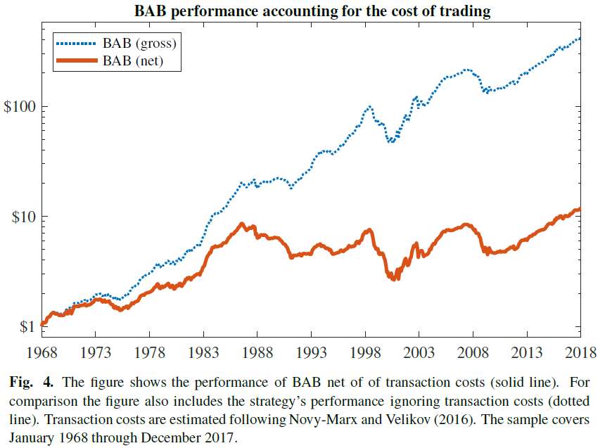
The results are hypothetical results and are NOT an indicator of future results and do NOT represent returns that any investor actually attained. Indexes are unmanaged, do not reflect management or trading fees, and one cannot invest directly in an index. Additional information regarding the construction of these results is available upon request.
As can be seen above, the overall performance of the BAB factor, after accounting for trading costs, significantly drops. Specifically, from the paper:
The figure shows that while accounting for transaction costs reduces BAB’s profitability more than 55%, the strategy still earns significant average net returns, 48 bps/month with a t-statistic of 3.30. BAB’s generalized alpha (Novy-Marx and Velikov 2016) relative to the Fama and French five-factor model, however, is only 16 bps/month and insignificant (t-statistic of 1.20; see Appendix C for details).
In addition, footnote 14 of the paper indicates that if one simply excluded the bottom decile of firms (i.e. kick out the micro-caps) and re-forms the BAB portfolio, the net returns (and alpha) are similar.
The results, discussed in Appendix C, are shown in Table 9 below.
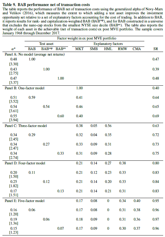
The results are hypothetical results and are NOT an indicator of future results and do NOT represent returns that any investor actually attained. Indexes are unmanaged, do not reflect management or trading fees, and one cannot invest directly in an index. Additional information regarding the construction of these results is available upon request.
As can be seen above, after transaction costs, the 5-factor alpha is insignificant for the 3 BAB models.
The paper additionally digs into the effect of the non-standard beta estimation procedure and the actual beta of BAB (is it actually market-neutral?), which interested readers can find in section 4 & 5.
Conclusion
Overall, this paper investigates the details of the BAB factor by taking a deep dive into the construction of the BAB factor. As can be seen, by Figure 2, the BAB factor is very similar to a portfolio long the top 1/3 (low beta) and short the bottom 1/3 (high beta) while equal-weighting the portfolio (and using leverage).
In addition, after accounting for transaction costs, the BAB factor has an insignificant 5-factor alpha.
So is all lost for the BAB factor?
No.
What the article highlights is that low volatility investing is another way to allocate towards the investment and profitability factors.
Even after transaction costs, the BAB factor has significant 1-factor alpha (using the CAPM regression) seen above in Table 9.
Thus, low-beta/low-volatility investing, in and of itself, is not a bad idea. However, if one already has an allocation towards the investment and profitability factors, a low-beta portfolio probably adds little to the portfolio.
Last, one may argue about the transaction cost assumptions embedded in the paper, thus leading one into another Novy-Marx/AQR argument on trading costs.
References[+]
| ↑1 | This is the high-level summary, not the exact details! |
|---|---|
| ↑2 | Note, one can vary the “1/3” and create another L/S factor return series, such as going long the top decile (1/10) and short the bottom decile (1/10). |
| ↑3 | Details are in the paper. |
| ↑4 | If interested in the math details, see the paper. |
| ↑5 | Note: I am assuming this is true, since the BAB factor uses leverage on the long portfolio, and deleverages the short portfolio, but I didn’t find it explicitly in the paper. |
| ↑6 |
 The results are hypothetical results and are NOT an indicator of future results and do NOT represent returns that any investor actually attained. Indexes are unmanaged, do not reflect management or trading fees, and one cannot invest directly in an index. Additional information regarding the construction of these results is available upon request. |
About the Author: Jack Vogel, PhD
—
Important Disclosures
For informational and educational purposes only and should not be construed as specific investment, accounting, legal, or tax advice. Certain information is deemed to be reliable, but its accuracy and completeness cannot be guaranteed. Third party information may become outdated or otherwise superseded without notice. Neither the Securities and Exchange Commission (SEC) nor any other federal or state agency has approved, determined the accuracy, or confirmed the adequacy of this article.
The views and opinions expressed herein are those of the author and do not necessarily reflect the views of Alpha Architect, its affiliates or its employees. Our full disclosures are available here. Definitions of common statistics used in our analysis are available here (towards the bottom).
Join thousands of other readers and subscribe to our blog.