Original: August, 2020
Updated: March, 2025
Overview
Digital signal processing (DSP), specifically the use of digital filters, is embedded in many indicators used by technical analysts to study and make trading decisions using time series of stock, bond, currency, commodity, and other financial asset prices. This analysis takes a look at several of the most commonly-used filters and indicators from a DSP perspective to illustrate their properties and limitations.
The filters and indicators analyzed are:
- moving average (MA)
- high pass moving average (HPMA)
- linear weighted moving average (LWMA)
- high pass linear weighted moving average (HPLWMA)
- exponential smoothing (ES)
- high pass exponential smoothing (HPES)
- time series momentum (TSMOM)
- averaged time series momentum (ATSMOM)
- moving average crossover (MAC)
- moving average convergence-divergence (MACD).
1. Financial Asset Prices and Time Series
Financial assets, such as stocks, bonds, currencies, and commodities, are priced as the result of trades made between buyers and sellers on exchanges, electronic trading systems, over the phone, etc. Prices are established and quoted when the buyer and seller agree on the value of the asset and execute a trade. Prices fluctuate in response to changes in supply and demand for the asset, market conditions, economic conditions, and other factors.
Trades are discrete events that can occur at different rates of time, depending on the type of asset, the type of market, etc. While trade-by-trade prices are available for many types of assets, technical analysts typically study price histories that are structured as data that is sampled at a uniform time interval, e.g., hourly, daily, weekly, or monthly. Data in this form are called discrete-time time series.
Characteristics of Financial Time Series
Financial time series by their nature are challenging to analyze because, in general, they display:
- volatility – financial time series tend to be “noisy”, i.e., with many rapid short-term fluctuations and jumps, making identifying the underlying trends and cycles difficult in real-time
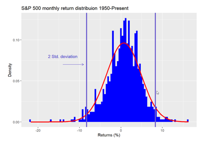
- non-normality – the mean and standard deviation of financial time series returns (i.e., the change in price over a specified period of time) do not conform to a normal probability distribution, e.g., observed return distributions are peaked with negative skewedness (skewness < 0) and “fat tails” (kurtosis > 3)
- non-stationarity – financial time series return probability distributions are not invariant under time shift, i.e., their means and variances change over time and cycles and trends do not persist.
2. Digital Filtering in Technical Analysis
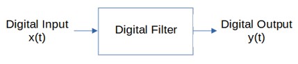
Digital filtering is widely used in electrical engineering, telecommunications, and other fields to process digital signals, e.g., to alter the features of the input signal in a particular way, which appears in the filter output.
Since financial time series data are digital by nature, various digital filtering techniques, such as moving averages and time series momentum (TSMOM), are used by technical analysts to transform and analyze them, e.g., to attenuate noise and identify trading opportunities presented by trends and cycles.
This section presents some basic concepts to aid in understanding how digital filters are designed and operate. Since, in the electrical engineering world, digital filters are categorized and viewed in terms of their effect on the frequencies of the signal passing through them, the concepts of time domain and frequency domain are described. More detailed discussion of digital filtering concepts can be found in various textbooks, such as [1] and [2].
The terms “filtering” and “smoothing” are often used interchangeably but are actually somewhat different. Assuming observations of the input are contaminated with noise:
- filtering – uses past and current observations to estimate the current state (i.e., causal)
- smoothing – uses past and current observations to estimate previous states (i.e., non-causal)
- prediction – uses past and current observations to forecast future states.
Frequency Measurement
For discrete-time signals containing cycles (i.e., sinusoidal-like patterns or waves), several different measurement conventions can be used:
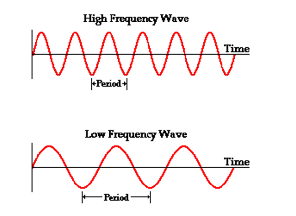
- Frequency – the number of cycles completed per time sample
Two common frequency measurements are:- f = the number of cycles per time sample (normalized frequency)
- ω = the number of radians per time sample where 2*π radians = 360o = 1 cycle (normalized angular frequency)
Relationships: - f = ω/(2*π)
- ω = 2*π*f
- Period – the number of time samples to complete one cycle
- P = the number of time samples to complete one cycle (normalized period)
Relationships: - P = 1/f
- P = 2*π/ω
- P = the number of time samples to complete one cycle (normalized period)
Measuring cycles using period, where the sampling rate can be hourly, daily, weekly, monthly, etc., is commonly used by and most familiar to technical analysts.
Time Domain and Frequency Domain
Financial time series that are structured as data sampled at a uniform time interval are referred to as being in the “time domain”. A graph in the time domain, such as a price chart, displays the time series value at each time sample. Technical analysts generally study data in the time domain, and the output of most technical analysis indicators is also calculated and displayed in the time domain.
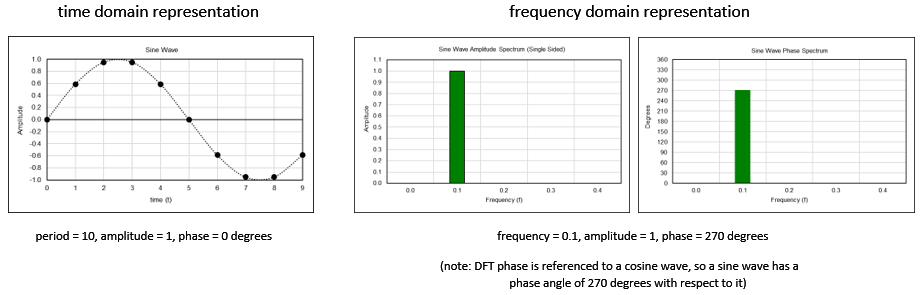
The Fourier theorem states that a general function, however complicated, may be expressed as the sum of sinusoidal functions or frequency components, each of which has a specific amplitude (a measure of maximum displacement from equilibrium) and phase (a measure of angular offset). While Fourier analysis was originally developed for continuous-time functions (e.g., analog signals), it is also applicable in a modified form to discrete-time functions (e.g., digital signals). Data represented in this way is referred to as being in the “frequency domain”.
Discrete-time time series can be converted from the time domain to the frequency domain using the Discrete Fourier Transform (DFT). The output of the Discrete Fourier Transform is the “frequency spectrum” of the time series, which is the amplitude and phase of each frequency component of the time series. Time series can be converted from the frequency domain to the time domain using the related Inverse Discrete Fourier Transform (IDFT). Details concerning spectral analysis and the DFT can be found in various textbooks and lecture notes, such as [1], [2], and [3]. See Appendix 1 for the DFT calculation.
Example: a 10 time sample period discrete-time sine wave represented in the time domain and in the frequency domain
Types of Filters
There are four basic types of filters:
- low pass – passes low frequencies (long periods) and attenuates high frequencies (short periods)
- high pass – passes high frequencies (short periods) and attenuates low frequencies (long periods)
- bandpass – passes frequencies (periods) within a specific range or bandwidth and attenuates the others
- bandstop – attenuates frequencies (periods) within a specific range or bandwidth and passes the others.
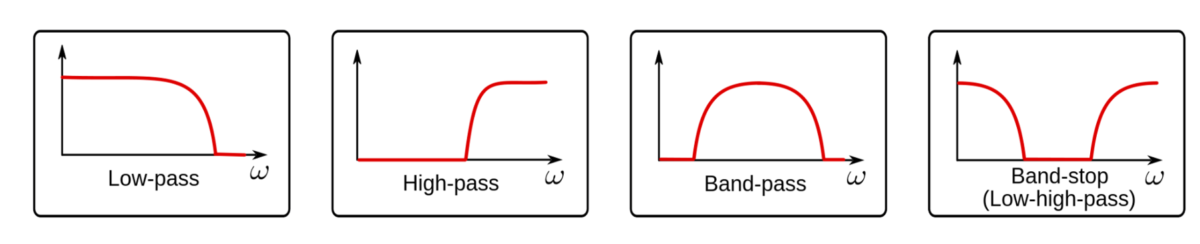
Since noise is associated with high frequencies (short periods), low pass filters are used in many technical analysis indicators. Bandpass filters are used to identify cycles in a particular frequency (period) range.
Some other types of filters used with financial time series are:
- differentiator – the filter output is proportional to the rate of change (i.e., the derivative with respect to time) of the input
- target tracking – used to calculate the position, velocity, and acceleration of a moving target; includes alpha-beta, alpha-beta-gamma, and Kalman filters.
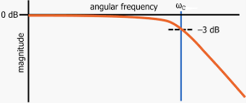
Cutoff Frequency
One technique used to understand and/or control the behavior of a filter is by knowing and/or setting the filter cutoff frequency. The cutoff frequency is the frequency at which the power of the filter output is reduced by a certain amount, relative to the power of the input.
A commonly-used cutoff frequency is one where the output power is one-half the input power:
- input power = input amplitude2 (i.e., input amplitude squared)
- output power = output amplitude2 (i.e., output amplitude squared)
- output power at one-half the input power:
- output power = ½*input power
- output amplitude = √½*input amplitude
- output magnitude = (output amplitude / input amplitude) = √½ = 0.7071
- conversion to decibels (dB): 20*log(0.7071) = -3.0104 dB.
Cutoff frequency is commonly denoted as ωc or fc. Cutoff period is denoted as Pc.
FIR and IIR Digital Filters
Digital filters can be implemented in two ways:
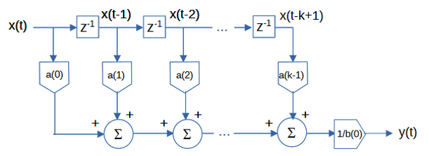
Finite impulse response (FIR) filters – The filter does not use feedback. The filter difference equation (also called the input-output equation) is non-recursive, i.e., it uses only current and past input values. The general FIR filter difference equation is:
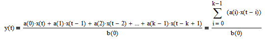
where
- k = number of filter input samples
- x(t-i) = filter input sample at integer time t-i for i = 0, 1, 2, …, k-1
- a(i) = filter coefficient of filter input x(t-i)
- y(t) = filter output at integer time t
- b(0) = filter coefficient of filter output y(t).
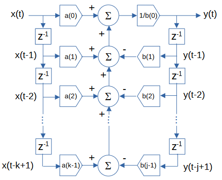
Infinite impulse response (IIR) filters – The filter uses feedback. The filter difference equation is recursive, i.e., it uses current and past input values as well as past output values. The general IIR filter difference equation is:

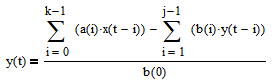
where
- k = number of filter input samples
- j = number of filter output samples
- x(t-i) = filter input sample at integer time t-i for i = 0, 1, 2, …, k-1
- a(i) = filter coefficient of filter input x(t-i)
- y(t-i) = filter output sample at integer time t-i for i = 0, 1, 2, …, j-1
- b(i) = filter coefficient of filter output y(t-i).
For the filters analyzed in this article, b(0) = 1.
The behavior of a filter, specifically its frequency response, is determined by the type of filter and the a(i) and b(i) filter coefficient values.
Filter Frequency Response
Frequency response measures the magnitude and phase of the filter output in response to a sinusoidal input of a given frequency ω. There are two components of frequency response:
- magnitude response |H(ω)| – the ratio of the amplitude of the filter output to the amplitude of the filter input at a given frequency ω
- phase response θ(ω) – the angular shift (i.e., time delay) of the filter output relative to the filter input at a given frequency ω, measured in radians or degrees.
See Appendix 2 for the calculation of frequency response.
Unit Pulse Response
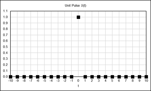
The response of a filter to a unit pulse input is called the “unit pulse response”. The unit pulse is denoted by δ(t), the Kronecker delta function, where:
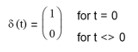
The unit pulse function is illustrated in the following graph.
The response of a filter to a unit pulse input completely defines the filter, i.e., both its time domain and frequency domain responses, since the unit pulse contains all frequencies. The filter response to a unit pulse input is represented by the unit pulse response coefficients h(i), where each h(i) coefficient denotes the filter response to the time-shifted unit pulse δ(t-i).
In the time domain, a filter operates on the input by multiplying the filter unit pulse response coefficients h(i) with the corresponding input values x(t-i) at each corresponding point in time, a procedure called “convolution”.
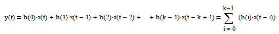
where
- k = number of filter unit pulse response coefficients
- x(t-i) = filter input sample at integer time t-i for i = 0, 1, 2, …, k-1
- h(i) = filter unit pulse response coefficient of filter input x(t-i)
- y(t) = filter output at integer time t.
See [1], for example, for additional details regarding the convolution operation.
For both FIR and IIR filters, the unit pulse response coefficients are used as the basis for calculating both the time and frequency domain responses. For FIR filters, the filter coefficients a(i) are equal to the unit pulse response coefficients h(i). Calculating the unit pulse response coefficients h(i) for IIR filters is more complex. See [4] for descriptions of several calculation methods.
In the frequency domain, the frequency spectrum of the filter output is obtained by multiplying the frequency spectrum of the input by the frequency response of the filter.
3. Notes on the Example Graphs
This article graphically illustrates representative time domain outputs and associated frequency domain magnitude and phase spectrums for the various filters and indicators, using common example parameter values.
The magnitude and phase spectrum graphs display the frequency response over the range 0 <= f <= 0.5 cycles per time sample on the horizontal scale. The lower limit f = 0 can be thought of as a wave of infinite length or as a steady direct current (DC) level. The upper limit f = 0.5 is called the “Nyquist frequency”, which is the highest frequency of a signal that can be recorded per time sample for the signal to be accurately reconstructable in the time domain.
Graphs showing the frequency response in terms of the period on the horizontal scale are also included since period is the measurement that is most commonly used by and familiar to technical analysts. The period graphs have a lower limit of 2 time samples, since the Nyquist frequency f = 0.5 corresponds to a period of P = 1/f = 2 time samples per cycle.
4. S&P 500 Time Domain and Frequency Domain for 2018-2019
Time Domain Representation
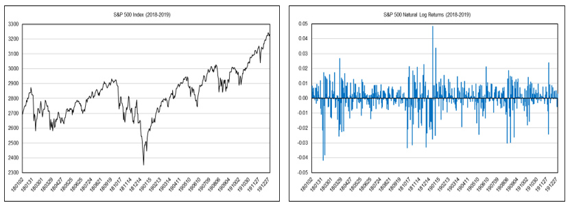
In this article, examples of the time domain output of the various filters and indicators are shown using price charts of the daily S&P 500 stock index closing values for 2018 and 2019, which includes 503 trading days.
Below left is a chart of the daily S&P 500 index closing values and below right is a chart of the daily natural log (i.e., continuously compounded) index returns r(t) = ln(x(t)/x(t-1)) where x(t) is the index value at integer time t corresponding to the date. The natural log returns are used to calculate the frequency spectrum.
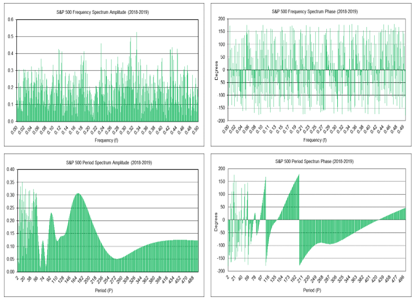
Frequency Domain Representation
Below upper left is a graph of the frequency spectrum magnitude of the S&P 500 daily natural log returns and below upper right is a graph of the frequency spectrum phase in degrees (please see the note regarding “phase wrap” in the “Moving Average Filter Frequency Response” section).
Below lower left is a graph of the period spectrum magnitude of the natural log returns and below lower right is a graph of the period spectrum phase in degrees. The period spectrum magnitude graph shows a number of short-cycle periods of up to approximately 55 days and two longer cycle periods of 95 and 169 days.
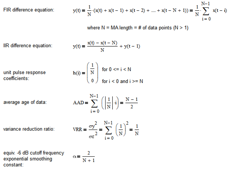
5. Moving Average (MA)
The moving average (MA) filter FIR difference equation is:
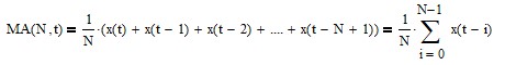
where N is the number of input data points included in the average, i.e., the moving average length (N > 1), and x(t) represents the price at integer time t. Moving average filter coefficients have equal value 1/N. The FIR difference equation coefficients sum to 1.0.
A moving average is a low pass FIR filter, i.e., it passes frequencies below the cutoff frequency and attenuates frequencies above the cutoff frequency. The moving average length N determines the frequency response of the filter. The cutoff frequency fc is inversely proportional to N (the cutoff period Pc is proportional to N).
MA can be calculated recursively in IIR form (requires proper initialization):
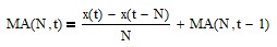
See Appendix 3 for additional details.
A commonly-used trading signal is generated when the current price crosses above (buy) or below (sell) the low pass moving average.
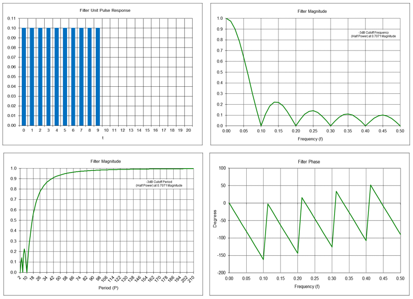
Moving Average Filter Frequency Response (N = 10)
Example: Moving average filter with length N = 10
MA(10, t) = [x(t) + x(t-1) + x(t-2) + x(t-3) + x(t-4) + x(t-5) + x(t-6) + x(t-7) + x(t-8) + x(t-9)] / 10
= 0.1*x(t) + 0.1*x(t-1) + 0.1*x(t-2) + 0.1*x(t-3) + 0.1*x(t-4) + 0.1*x(t-5) + 0.1*x(t-6) + 0.1*x(t-7) + 0.1*x(t-8) + 0.1*x(t-9)
Passes frequencies below the -3 dB cutoff frequency fc of approximately 0.044, which corresponds to a cutoff period Pc of approximately 22.5 time samples.
As can be seen in the frequency magnitude graph, a moving average filter of length N = 10 completely suppresses frequencies of 0.1, 0.2, 0.3, 0.4, and 0.5, which correspond to periods of 10, 5, 3.333, 2.5, and 2 time samples, respectively. Suppression occurs because, for example, the average value of a 10 time sample period sine wave over 10 time samples is zero, the average value of two 5 time sample period sine waves over 10 time samples is zero, etc.
Note: In the filter phase graphs in this article, phase values are constrained to the range of -180 degrees to +180 degrees. When the actual phase value is outside this range, the phase value is increased or decreased by a multiple of 360 degrees to put the phase value back within the +/-180 degree range. This is called “phase wrap” and results in the appearance of a zig-zag line, but each zig-zag line segment is actually a continuation of the previous line segment.
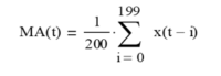
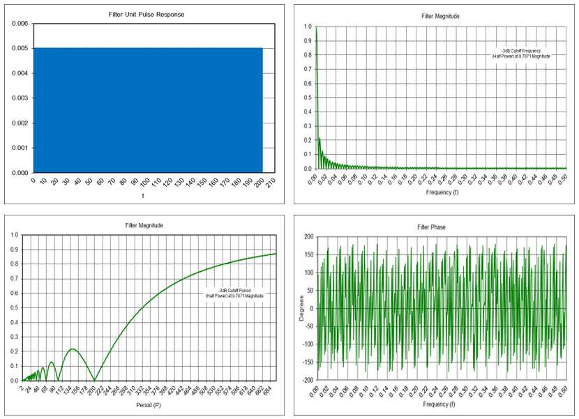
Moving Average Filter Frequency Response (N = 200)
Example: Moving average filter with N = 200, which is a popular moving average length used with daily data.
Passes frequencies below the -3 dB cutoff frequency fc of approximately 0.002215, which corresponds to a cutoff period Pc of approximately 451.5 time samples.
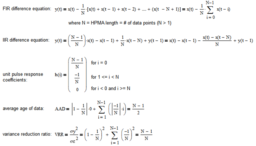
6. High Pass Moving Average (HPMA)
Subtracting a moving average, which is a low pass FIR filter, from the input results in a high pass FIR filter, i.e., frequencies above the cutoff frequency are passed and frequencies below the cutoff frequency are attenuated. The high pass moving average (HPMA) filter FIR difference equation is:
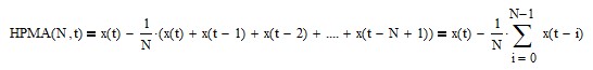
The FIR difference equation coefficients sum to 0.0.
The high pass moving average filter IIR difference equation (requires proper initialization) is:
See Appendix 4 for additional details.
The high pass moving average crosses above (below) zero at the same time as the current price crosses above (below) the low pass moving average.
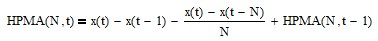
Example: High pass moving average filter with length N = 10
HPMA(10, t) = x(t) – [x(t) + x(t-1) + x(t-2) + x(t-3) + x(t-4) + x(t-5) + x(t-6) + x(t-7) + x(t-8) + x(t-9)] / 10
= 0.9*x(t) – 0.1*x(t-1) – 0.1*x(t-2) – 0.1*x(t-3) – 0.1*x(t-4) – 0.1*x(t-5) – 0.1*x(t-6) – 0.1*x(t-7) – 0.1*x(t-8) – 0.1*x(t-9)
Passes frequencies above the -3 dB cutoff frequency fc of approximately 0.027, which corresponds to a cutoff period Pc of approximately 37.2 time samples.
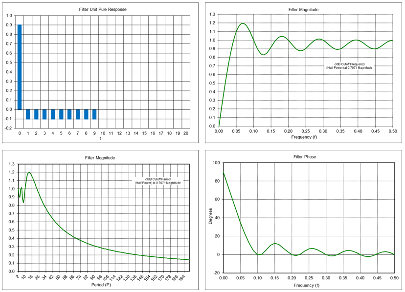
The chart below shows the MA and HPMA filters applied to the daily S&P 500 index for the years 2018-2019. The trading signals generated in the time domain are indicated by the lines at the bottom of the chart.
The results are hypothetical results and are NOT an indicator of future results and do NOT represent returns that any investor actually attained. Indexes are unmanaged, do not reflect management or trading fees, and one cannot invest directly in an index.
7. Linear Weighted Moving Average (LWMA)
The linear weighted moving average (LWMA) filter difference equation is:
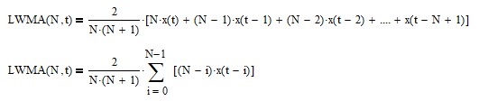
where N is the number of input data points included in the average, i.e., the linear weighted moving average length (N > 1). The filter coefficients are linearly weighted with the greatest weights placed on the most recent input values. The FIR difference equation coefficients sum to 1.0.
A linear weighted moving average is a low pass FIR filter, i.e., it passes frequencies below the cutoff frequency and attenuates frequencies above the cutoff frequency. The value of the linear weighted moving average length N determines the frequency response of the filter. The cutoff frequency fc is inversely proportional to N (the cutoff period Pc is proportional to N).
LWMA can be calculated recursively in IIR form (requires proper initialization):
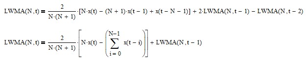
See Appendix 5 for additional details.
A commonly-used trading signal is generated when the current price crosses above (buy) or below (sell) the low pass linear weighted moving average.
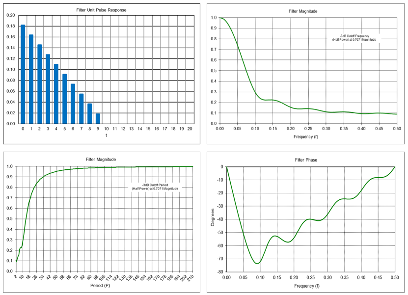
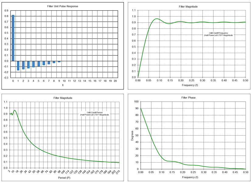
LWMA Filter Frequency Response (N = 10)
Example: Linear weighted moving average filter with length N = 10 (note: coefficients shown are rounded)
LWMA(10, t) = 0.1818*x(t) + 0.1636*x(t-1) + 0.1455*x(t-2) + 0.1273*x(t-3) + 0.1091*x(t-4) + 0.0909*x(t-5) + 0.0727*x(t-6) + 0.0545*x(t-7) + 0.0364*x(t-8) + 0.0182*x(t-9)
Passes frequencies below the -3 dB cutoff frequency fc of approximately 0.053, which corresponds to a cutoff period Pc of approximately 18.8 time samples.
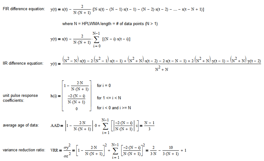
8. High Pass Linear Weighted Moving Average (HPLWMA)
Subtracting a linear weighted moving average from the input results in a high pass FIR filter, i.e., frequencies above the cutoff frequency are passed and frequencies below the cutoff frequency are attenuated. The high pass linear weighted moving average (HPLWMA) filter FIR difference equation is:
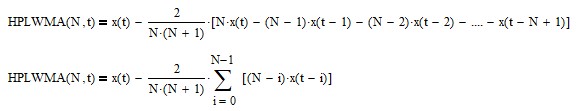
The FIR difference equation coefficients sum to 0.0.
The high pass linear weighted moving average filter IIR difference equation (requires proper initialization) is:

See Appendix 6 for additional details.
The high pass linear weighted moving average crosses above (below) zero at the same time as the current price crosses above (below) the low pass linear weighted moving average.
Example: High pass linear weighted moving average filter with length N = 10 (note: coefficients shown are rounded)
HPLWMA(10, t) = x(t) – [0.1818*x(t) + 0.1636*x(t-1) + 0.1455x(t-2) + 0.1273*x(t-3) + 0.1091*x(t-4) + 0.0909*x(t-5) + 0.0727*x(t-6) + 0.0545*x(t-7) + 0.0364*x(t-8) + 0.0182*x(t-9)]
= 0.8182*x(t) – 0.1636*x(t-1) – 0.1455*x(t-2) – 0.1273*x(t-3) – 0.1091*x(t-4) – 0.0909*x(t-5) – 0.0727*x(t-6) – 0.0545*x(t-7) – 0.0364*x(t-8) – 0.0182*x(t-9)
Passes frequencies above the -3 dB cutoff frequency fc of approximately 0.043, which corresponds to a cutoff period Pc of approximately 23.3 time samples.
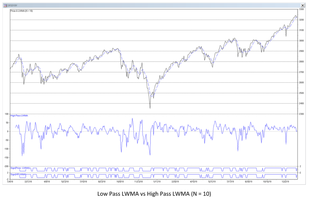
The chart below shows the LWMA and HPLWMA filters applied to the daily S&P 500 index for the years 2018-2019. The trading signals generated in the time domain are indicated by the lines at the bottom of the chart.
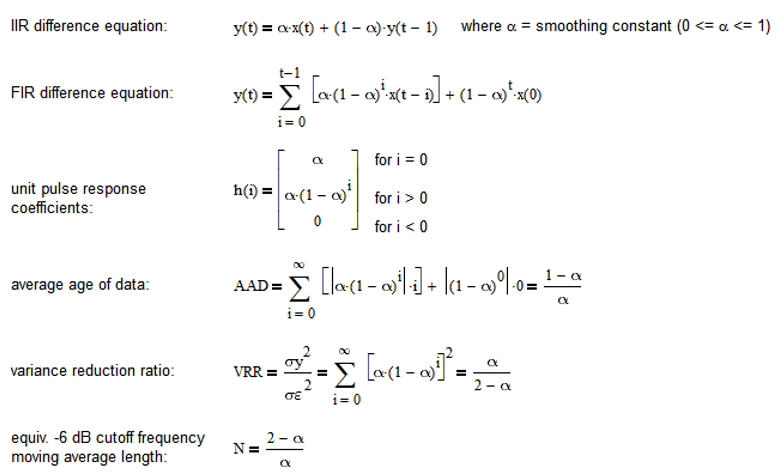
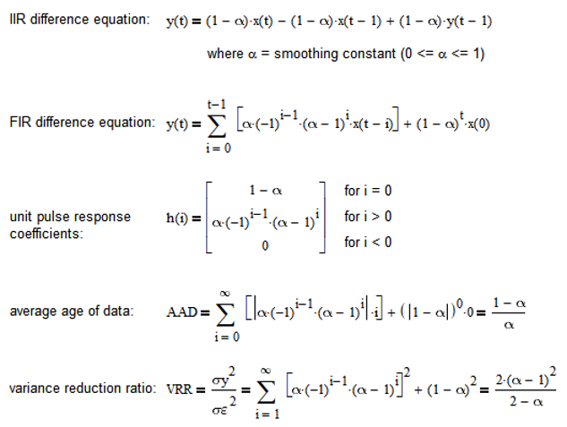
9. Exponential Smoothing (ES)
The exponential smoothing (ES) filter IIR difference equation is:
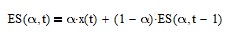
where α is the smoothing constant (0 <= α <= 1). The filter smoothing constant α is applied to the current input value and (1 – α) is applied to the previous filter output value.
Exponential smoothing is a low pass IIR filter, i.e., it passes frequencies below the cutoff frequency and attenuates frequencies above the cutoff frequency. The value of the smoothing constant α determines the frequency response of the filter. The cutoff frequency fc is proportional to α (the cutoff period Pc is inversely proportional to α).
ES can be calculated non-recursively in FIR form:
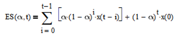
The FIR difference equation coefficients sum to 1.0. See Appendix 7 for additional details.
A commonly-used trading signal is generated when the current price crosses above (buy) or below (sell) the low pass exponential smoothing.
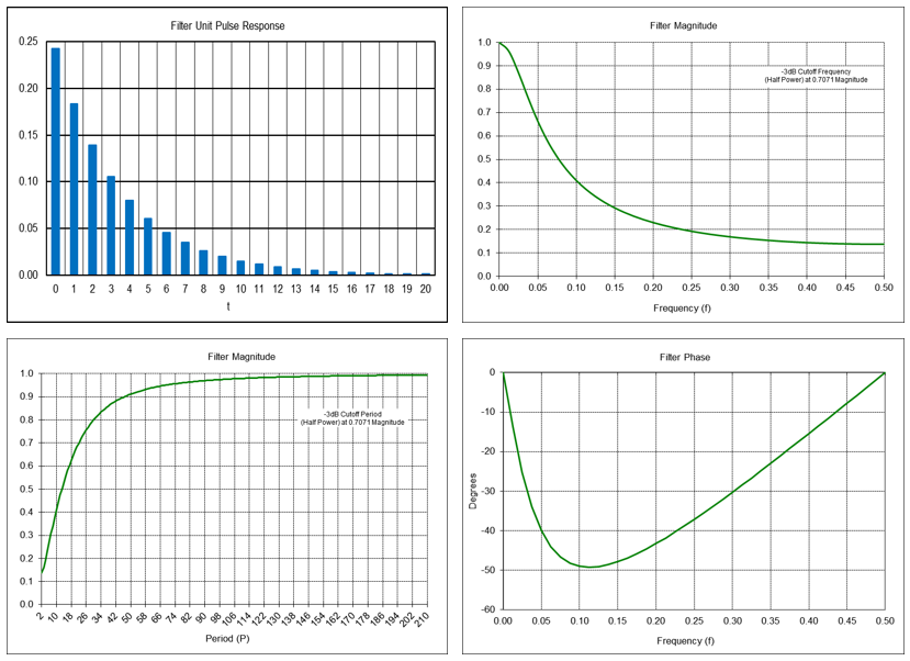
Exponential Smoothing Filter Frequency Response (α = 0.2425)
Example: exponential smoothing filter with smoothing constant α = 0.2425
ES(0.2425, t) = 0.2425*x(t) + 0.7575*ES(0.2425, t-1)
Passes frequencies below the -3 dB cutoff frequency fc of approximately 0.044 (i.e., the same cutoff frequency as a moving average filter of length N = 10), which corresponds to a cutoff period Pc of approximately 22.5 time samples. Note: The unit pulse response graph is limited to the first 21 time steps.
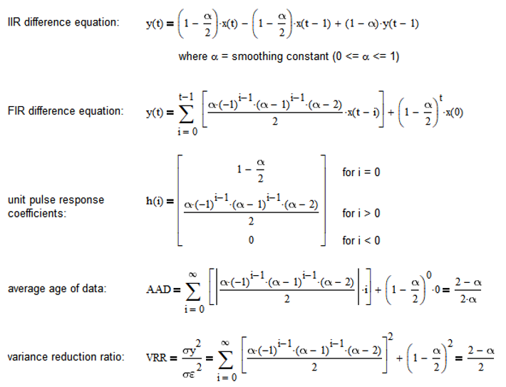
10. High Pass Exponential Smoothing (HPES)
Subtracting an exponential smoothing from the input results in a high pass IIR filter, i.e., frequencies above the cutoff frequency are passed and frequencies below the cutoff frequency are attenuated. The high pass exponential smoothing (HPES) filter IIR difference equation is:

See Appendix 8a for additional details.
The filter gain can be adjusted so that the maximum magnitude frequency response of the filter is 1.0 (0 dB), resulting in the difference equation:
See Appendix 8b for additional details.
The high pass exponential smoothing crosses above (below) zero at the same time as the current price crosses above (below) the low pass exponential smoothing.
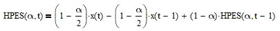
Example: High pass gain-adjusted exponential smoothing filter with α = 0.2425
HPES(0.2425, t) = 0.87875*x(t) – 0.87875*x(t-1) + 0.7575*HPES(0.2425, t-1)
Passes frequencies above the -3 dB cutoff frequency fc of approximately 0.044, which corresponds to a cutoff period Pc of approximately 22.5 time samples. Note: The unit pulse response graph is limited to the first 21 time steps.
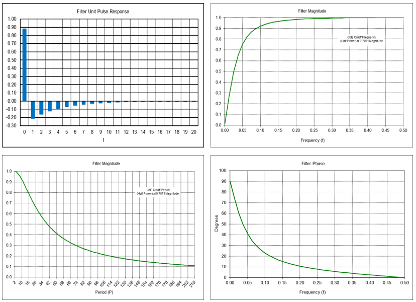
The chart below shows the ES and HPES filters applied to the daily S&P 500 index for the years 2018-2019. The trading signals generated in the time domain are indicated by the lines at the bottom of the chart.
11. Properties of MA, LWMA and ES Filters
Underlying Process Model
Moving average, linear weighted moving average, and exponential smoothing filters are low pass filters, which are modeled on the assumption that the underlying process has a locally constant mean value (i.e., with no trends or cycles) which is contaminated with normally distributed random noise ε(t) where ε(t) ~ N(0, σε2):
first order process – mean a: x(t) = a + ε(t)
Low pass filters are designed to estimate the mean value a by attenuating the random noise ε(t).
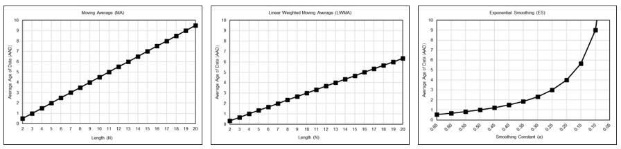
Average Age of Data
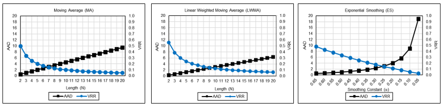
An important metric for analyzing and comparing the time domain characteristics of a filter is the average age of the data (AAD) passing through the filter, which was defined by Brown in [5]. AAD can generally be calculated as the sum of the absolute values of the time-weighted filter unit pulse response coefficients h(i):
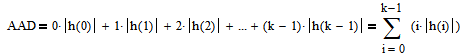
where k = number of filter unit pulse response coefficients and |h(i)| = absolute value of the unit pulse response coefficient for i = 0, 1, 2, …, k-1.
The graphs below show the AADs of the MA, LWMA, and ES filters over a range of parameter values. See Appendices 3, 5, and 7, respectively, for the AAD calculation for those filters.
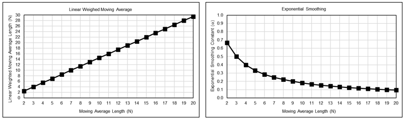
Low Pass Filters with Equivalent AAD
AAD can be used as the basis to calculate equivalent filter parameter values for different filter designs, e.g., the N and α values that result in the equivalent AAD for each filter design. This method is commonly used in the technical analysis literature and equates filters at their corresponding -6 dB (quarter power) cutoff frequencies. For a moving average filter with length NMA, the AAD-equivalent LWMA N and ES α are:
- NLWMA = (3*NMA – 1) / 2
- αES = 2 / (NMA + 1)
The parameter equivalences across a range of moving average lengths N are shown graphically below.
Variance Reduction Ratio
For time series containing normally distributed random noise ε(t) ~ N(0, σε2), the variance reduction ratio (VRR) of a filter measures the reduction in the variance of the filter output y(t), i.e., the noise, relative to the variance of the filter input and is calculated by summing the squares of the filter unit pulse response coefficients h(i) [5]. VRR is the ratio of the filter output variance to the input variance:
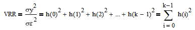
where k = number of filter unit pulse response coefficients and h(i) = unit pulse response coefficient for i = 0, 1, 2, …, k-1. Note that this calculation is equivalent to the Herfindahl-Hirschman Index [6]. The smaller the ratio, the greater the noise reduction. For example, VRR = 0 indicates complete noise reduction, whereas VRR = 1 indicates no noise reduction.
The graphs below illustrate the trade-off between AAD and VRR for the MA, LWMA, and ES filters across a range of filter parameter values. In general, the larger the length N or the smaller the smoothing constant α used in a filter, the smaller the VRR but the greater the AAD. See Appendices 3, 5, and 7, respectively, for the VRR calculation for these filters.
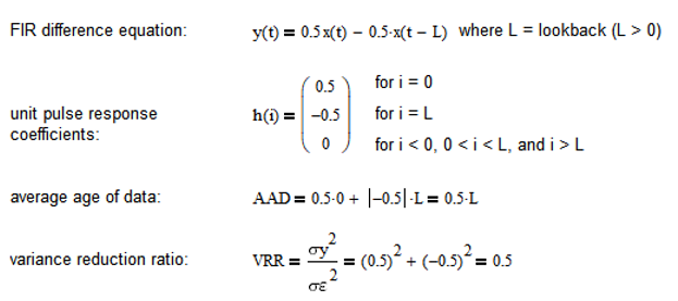
12. Time Series Momentum (TSMOM)
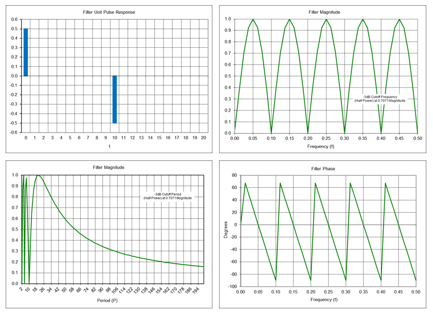
The time series momentum (TSMOM) filter FIR difference equation is:
where L is the integer time sample lookback (L > 0) and G is the filter gain adjustment (G > 0). TSMOM calculates the difference between two data points that are separated by the lookback, which is a fixed number of integer time samples. The FIR difference equation coefficients sum to 0.0. See Appendix 9 for additional details.
TSMOM is the simplest FIR differentiator, since it only uses two input data points. When used with monthly financial time series, for example, the lookback is typically set to 10 or 12 months. The filter gain adjustment G is often set to 1.0 but should be set to 0.5 so that the maximum magnitude frequency response of the filter is 1.0 (0 dB).
A commonly-used trading signal is generated when TSMOM changes sign, i.e., crosses above (buy) or below (sell) zero.
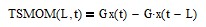
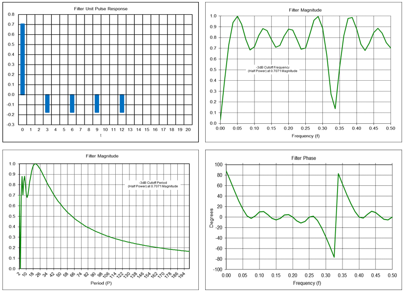
TSMOM Filter Frequency Response (L = 10)
Example: TSMOM filter with lookback L = 10
TSMOM(10, t) = 0.5*x(t) – 0.5*x(t-10)
Completely passes frequencies of 0.05, 0.15, 0.25, 0.35, and 0.45, which correspond to periods of 20, 6.667, 4, 2.857, and 2.222 time samples, respectively. Completely suppresses frequencies of 0.1, 0.2, 0.3, 0.4, and 0.5, which correspond to periods of 10, 5, 3.333, 2.5, and 2 time samples, respectively, and are the same as a moving average filter of length N = 10, except that TSMOM also suppresses f = 0.0, which is characteristic of a differentiator.
The chart below shows the TSMOM filter applied to the daily S&P 500 index for the years 2018-2019. The trading signals generated in the time domain are indicated by the line at the bottom of the chart.
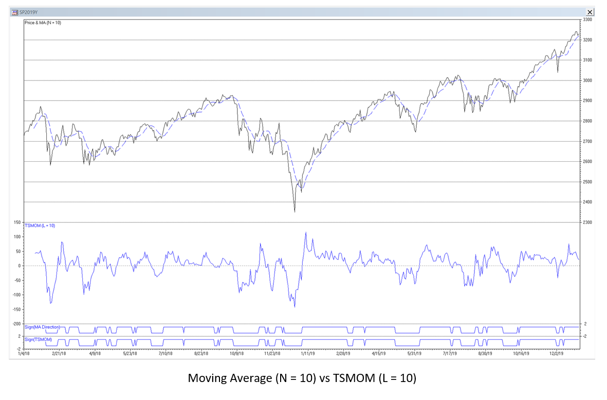
Mathematical Relationship Between MA and TSMOM
MA and TSMOM filters have different behaviors but are mathematically related. If the TSMOM lookback L is set equal to the moving average filter length N so that L = N:
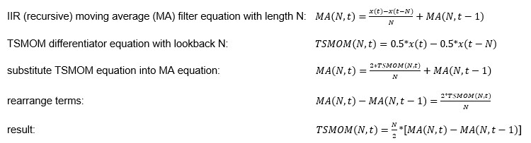
Comments on TSMOM
TSMOM changes sign when the comparable MA passes an inflection point, i.e., the MA changes direction. The equivalence of the trading signals generated by TSMOM crossing the zero line and MA changing direction is illustrated by the two lines at the bottom of the price chart above.
Price can potentially cross the MA before the MA itself changes direction, so price crossings can sometimes give earlier trading signals than TSMOM but, as a consequence, also generate more “whipsaw” trades that produce losses.
13. Averaged Time Series Momentum (ATSMOM)
Some TSMOM-based systems use an average of several TSMOM filters with different lookbacks. This type of filter can be analyzed by averaging the coefficients of the filters. The gain adjustment G can be used to normalize the resulting averaged TSMOM (ATSMOM) filter coefficients so that the maximum magnitude frequency response of the filter is 1.0 (0 dB).
Example: average of four TSMOM filters with 3, 6, 9, and 12 time sample lookbacks
L = 3: TSMOM(3, t) = x(t) – x(t-3)
L = 6: TSMOM(6, t) = x(t) – x(t-6)
L = 9: TSMOM(9, t) = x(t) – x(t-9)
L = 12: TSMOM(12, t) = x(t) – x(t-12)
gain-adjusted average:
ATSMOM(3, 6, 9, 12, t) = G*[4*x(t) – x(t-3) – x(t-6) – x(t-9) – x(t-12)]/4 = G*[x(t) – 0.25*x(t-3) – 0.25*x(t-6) – 0.25*x(t-9) – 0.25*x(t-12)]
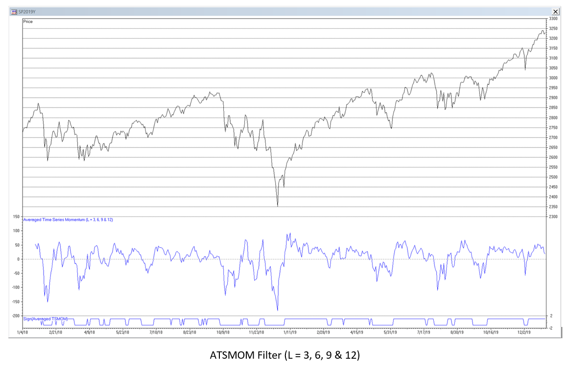
ATSMOM Filter Frequency Response (L = 3, 6, 9 & 12)
Example: ATSMOM filter with lookbacks L = 3, 6, 9 and 12. The gain adjustment is set to G = 0.7043 so that the maximum magnitude frequency response of the filter is 1.0 (0 dB).
ATSMOM(3, 6, 9, 12, t) = 0.7043*[x(t) – 0.25*x(t-3) – 0.25*x(t-6) – 0.25*x(t-9) – 0.25*x(t-12)]
= 0.7043*x(t) – 0.176075*x(t-3) – 0.176075*x(t-6) – 0.176075*x(t-9) – 0.176075*x(t-12)
Completely passes frequencies of approximately 0.05, 0.29, and 0.385, which correspond to periods of approximately 20, 3.45, and 2.6 time samples, respectively.
The chart below shows the ATSMOM filter applied to the daily S&P 500 index for the years 2018-2019. The trading signals generated in the time domain are indicated by the line at the bottom of the chart.
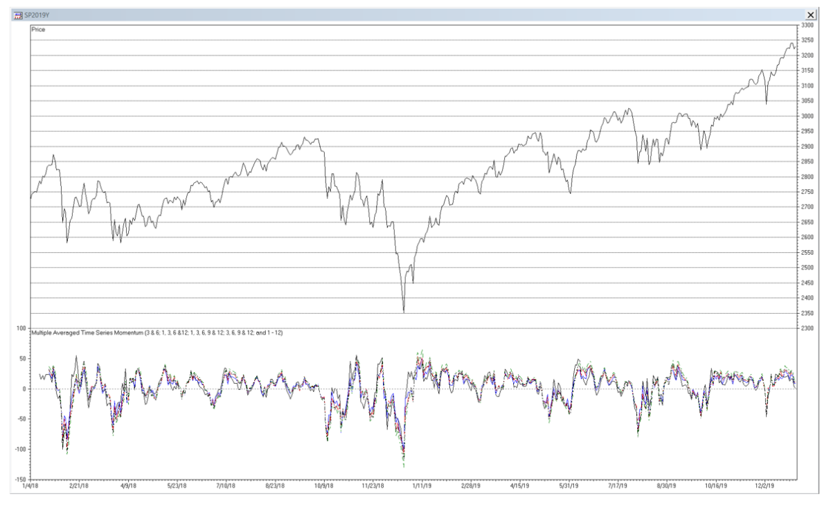
Comments on ATSMOM
Some technical analysts use different lookback combinations, such as 3 and 6; 1, 3, 6 and 12; 1, 3, 6, 9 and 12; 3, 6, 9 and 12; and even 1 through 12. The smaller lookbacks are included to capture shorter-term movements, whereas the larger lookbacks are included to capture long-term momentum.
The frequency response of an ATSMOM filter can vary widely, depending on the number and corresponding lookbacks of the individual filters included. However, the ones listed above produce similar-looking outputs since they include similar lookbacks.
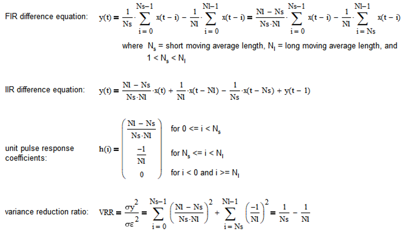
14. Moving Average Crossover (MAC)
Moving average crossover (MAC) uses the difference between two moving averages. One moving average has a short length Ns and the other a longer length Nl:
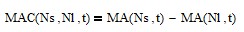
where 1 < Ns < Nl.
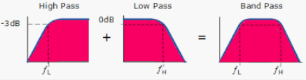
Moving average crossover is a type of bandpass FIR filter, passing frequencies between low (fL) and high (fH) cutoff frequencies, called the bandwidth (Δf = fH – fL). The filter has a center (also called “resonant”) frequency (f0) located between the two cutoffs, which the filter passes at maximum power. The bandwidth and center frequency are determined by the two moving average lengths Ns and Nl. The FIR difference equation coefficients sum to 0.0. See Appendix 10 for additional details.
MAC illustrates that a bandpass filter can be implemented by subtracting a low pass filter with a lower cutoff frequency from a low pass filter with a higher cutoff frequency. (Note that, as was mentioned earlier, subtracting a low pass filter from the input results in a high pass filter.)
MAC can be calculated recursively in IIR form (requires proper initialization):

A commonly-used trading signal is generated when the short moving average MA(Ns, t) crosses above (buy) or below (sell) the long moving average MA(Nl, t).
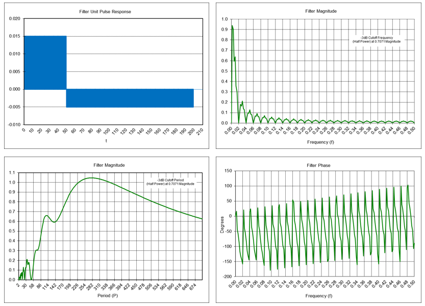
MAC Frequency Response (Ns = 50 & Nl = 200)
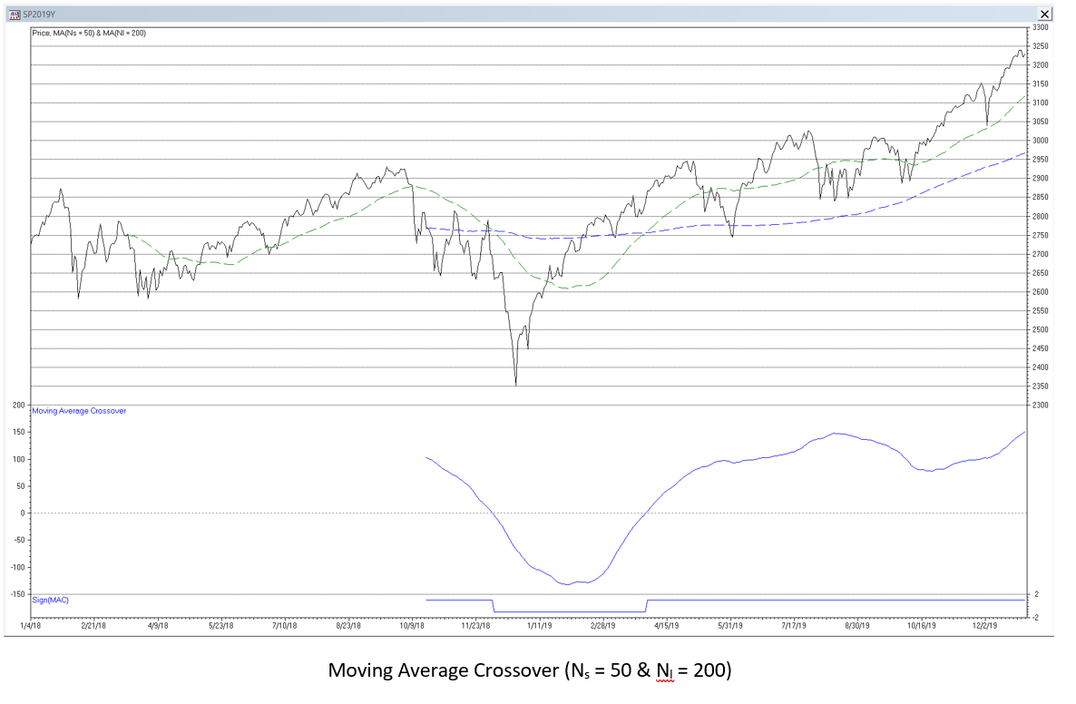
A popular moving average crossover uses short MA length Ns = 50 days and long MA length Nl = 200 days. The “Golden Cross”, used to identify a bull market, occurs when the 50-day MA moves above the 200-day MA. The “Death Cross”, used to identify a bear market, occurs when the 50-day MA moves below the 200-day MA.
Example: Moving average crossover filter where Ns = 50 and Nl = 200:
MAC(50, 200, t) = MA(50, t) – MA(200, t)
The -3 dB short cutoff period Pcs is approximately 166 time samples, the -3 dB long cutoff period Pcl is approximately 604 time samples, and the center (resonant) period P0 is approximately 279 time samples.
The chart below shows the MAC filter applied to the daily S&P 500 index for the years 2018-2019. The trading signals generated in the time domain are indicated by the line at the bottom of the chart.
15. Moving Average Convergence-Divergence (MACD)
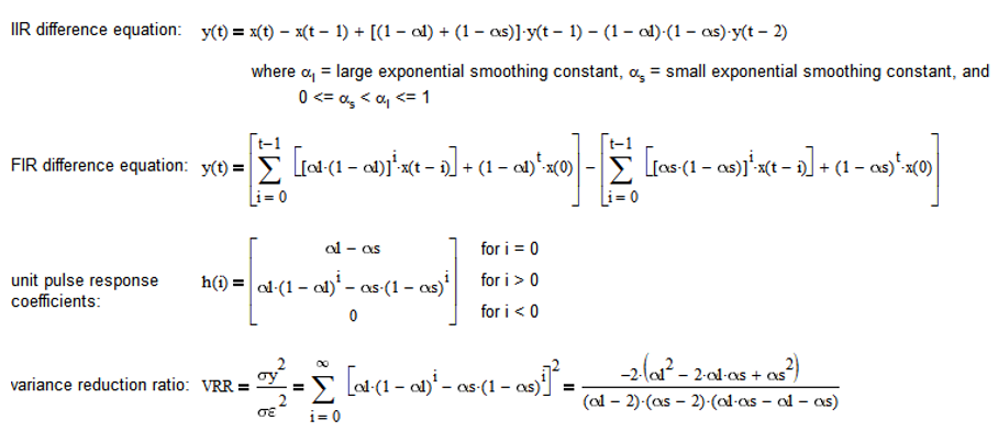
The term “moving average convergence-divergence” is a bit of a misnomer, since it is actually calculated using the difference between two exponential smoothing filters, not two moving averages. As a result of this naming convention, MACD parameters are usually specified using moving average lengths. The result is one exponential smoothing using a large smoothing constant αl (i.e., based on the short MA length Ns) and the other using a smaller smoothing constant αs (i.e., based on the long MA length Nl):
where 1 < Ns < Nl and, consequently, 0 < αs < αl <= 1.
MACD is a type of bandpass IIR filter, passing frequencies between low (fL) and high (fH) cutoff frequencies, called the bandwidth (Δf = fH – fL). The filter has a center (also called “resonant”) frequency (f0), which the filter passes at maximum power. The bandwidth and center frequency are determined by the two smoothing constants αl and αs.
MACD can be calculated recursively in IIR form (requires proper initialization):

where G is the filter gain adjustment where G > 0 and is usually set to 1.0.
See Appendix 11 for additional details. Note that the FIR difference equation coefficients sum to 0.0.
MACD can be interpreted in several ways. One type of MACD trading signal is generated when ES(αl, t) crosses above (buy) or below (sell) ES(αs, t). Another type of MACD trading signal uses the difference between the two exponential smoothing filters (called the “MACD line”) and additionally smoothing the result using another exponential smoothing filter to generate a “signal line”. The trading signal is generated when the MACD line crosses above (buy) or below (sell) the signal line.
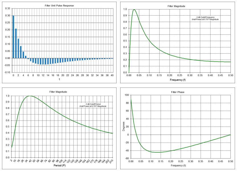
MACD Frequency Response (αl = 0.2067 & αs = 0.1015)
A popular MACD configuration is to set αl equivalent to a moving average length of 12 days and αs equivalent to a moving average length of 26 days.
Example: Moving average convergence-divergence filter where MA Ns = 12 and MA Nl = 26
Note: The formula α = 2/(N + 1) is usually used to convert a MA length N to the equivalent ES smoothing constant α. This formula actually equates the two at their corresponding -6 dB (quarter power) cutoff frequencies. To maintain consistency with the other examples, smoothing constants that specify the -3 dB cutoff frequency are used here instead: αl = 0.2067 and αs = 0.1015.
MACD(12, 26, t) = ES(0.2067, t) – ES(0.1015, t)
Setting the gain adjustment G = 0.2863 so that the maximum frequency magnitude response of the filter is 1.0 (0 dB) at the center frequency of approximately 40 time samples, the -3 dB short cutoff period Pcs is approximately 15 time samples and the -3 dB long cutoff period Pcl is approximately 101 time samples. Note: The unit pulse response graph is limited to the first 41 time steps.
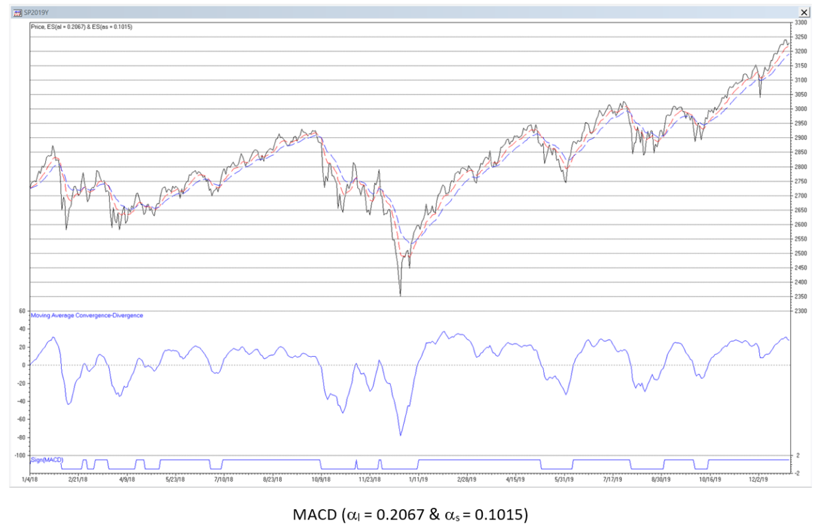
The chart below shows the MACD filter applied to the daily S&P 500 index for the years 2018-2019. The trading signals generated in the time domain are indicated by the line at the bottom of the chart.
Comments on MACD
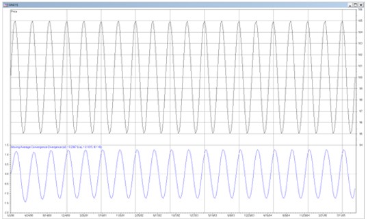
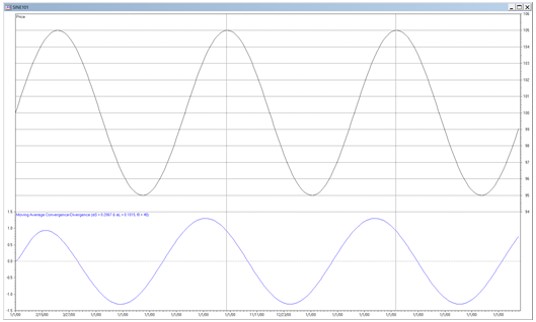
Since MACD is a bandpass filter, it is “tuned” to a specific center (resonant) frequency or period, based on the filter coefficients, and has an associated phase response. As a result, if the input time series cycle period is less than the center period of the filter, the filter output will peak (trough) after the input time series cycle peak (trough). This effect is shown in the graph below where a 15-period sine wave input, shown in the upper part, is plotted against the output of a MACD filter with αl = 0.2067 and αs = 0.1015 that has a center period of 40, shown in the lower part.
Conversely, if the input time series cycle period is greater than the center period, the filter output will peak (trough) before the input time series peak (trough). This effect is shown in the graph below where a 101-period sine wave input, shown in the upper part, is plotted against the output of a MACD filter with αl = 0.2067 and αs = 0.1015 that has a center period of 40, shown in the lower part.
A mismatch between the phases of the filter input and output due to the phase response of the filter produces what technical analysts call “divergence”, where the direction of the price “diverges” from the direction of the MACD line. Divergence is often interpreted as a predictive signal but is actually just an artifact of the filter phase response.
16. General Comments on Using Digital Filters
Pros and cons of FIR versus IIR filters:
- FIR filters generally have a more linear phase response, but the filter calculation can be more complex, e.g., due to usually requiring more memory of the previous input values.
- IIR filters have non-linear phase response, which can cause output distortion, but the filter calculation is usually simpler, e.g., generally not requiring as much memory of the previous input values.
Since financial time series contain trends, it is more appropriate to use filters which are designed to model underlying processes that contain trends and are contaminated with random normally distributed noise ε(t) ~ N(0, σε2):
- second order process – mean a and linear trend b: x(t) = a + b*t + ε(t)
- third order process – mean a, linear trend b, and quadratic trend c: x(t) = a + b*t + ½*c*t2 + ε(t)
Examples of such filters include double moving average, double exponential smoothing, and alpha-beta tracking filters [7], which are based on second order process models, and triple moving average, triple exponential smoothing, and alpha-beta-gamma tracking filters [8], which are based on third order process models.
Since financial time series are non-stationary with means and variances that change over time, the use of filters with fixed parameters will not perform well at all times for trading purposes. As a result, filter coefficients that are “fitted” to a particular portion of a time series history will not generally produce good results in the future. Some types of filters, called “adaptive filters”, employ techniques to modify the filter coefficient values over time in response to changes in the characteristics of the input [9] [10].
17. Forecasting Accuracy
When using MA, LWMA, or ES filters to estimate current values or forecast future values of a process, large N and small α values give more accurate estimates, assuming that the underlying process mean is stable, whereas small N and large α values give more responsive estimates if the underlying process mean changes.
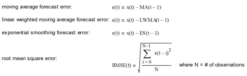
One measure that can be used to evaluate an appropriate N or α value to use with a particular time series is to calculate the root mean square error (RMSE) of the filter forecasts over a sample of observations. The forecast error is the difference between the current input value and the forecast. For low pass filters, the forecast is the previous filter output value since they do not model trends.
In general, the N or α value that produces the minimum RMSE can be helpful in determining a useful setting. However, if these low pass filters, which are modeled on a first order process, are applied to time series that contain trends, the minimum RMSE value in that case will generally occur for N = 2 (the minimum value for MA and LWMA) and α = 1.0 (the maximum value for ES), and the RMSE will increase as N increases and as α decreases. RMSE can be used to better effect with more complex filters that are designed for time series containing trends.
Acknowledgements
I would like to thank Larry Stabile for reviewing this article and providing many helpful comments and suggestions.
Appendix 1 – Discrete Fourier Transform
Digital signals and time series can be analyzed in the frequency domain using the Discrete Fourier Transform (DFT). The DFT calculation is:
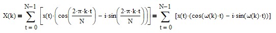
where
- X(k) = frequency component k for k = 0, 1, 2, …, N-1
- N = number of samples of the signal or time series x(t)
- x(t) = signal or time series sample at integer time t = 0, 1, 2, …, N-1
- i = √-1
- ω(k) = 2*π*k/N = frequency of frequency component X(k) in radians.
Frequency ω(k) in radians can be converted to frequency f(k) using f(k) = ω(k)/(2*π) or to period P(k) using P(k) = 2*π/ω(k).
The amplitude |X(k)| of frequency component k is:
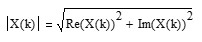
where Re(X(k)) is the real part of X(k) and Im(X(k)) is the imaginary part of X(k).
The phase θ(X(k)) of frequency component k in radians is:
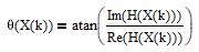
Phase response θ(X(k)) values can be converted from radians to degrees by multiplying by 180/π.
Appendix 2 – Frequency Response
The frequency response H(ω) of a filter to a sinusoidal input with frequency ω radians is:
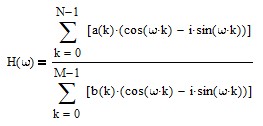
where
- N = number of a(k) filter coefficients
- M = number of b(k) filter coefficients
- i = √-1.
The magnitude response |H(ω)| is:
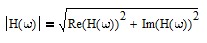
where Re(H(ω)) is the real part of H(ω) and Im(H(ω)) is the imaginary part.
The phase response θ(ω) is:
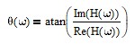
Phase response θ(w) values can be converted from radians to degrees by multiplying by 180/π.
Appendix 3 – Moving Average (MA) Equations
Appendix 4 – High Pass Moving Average (HPMA) Equations
Appendix 5 – Linear Weighted Moving Average (LWMA) Equations

Appendix 6 – High Pass Linear Weighted Moving Average (HPLWMA) Equations
Appendix 7 – Exponential Smoothing (ES) Equations
Appendix 8a – High Pass Exponential Smoothing (HPES) Equations (Unadjusted Gain)
Appendix 8b – High Pass Exponential Smoothing (HPES) Equations (Adjusted Gain)
Appendix 9 – Time Series Momentum (TSMOM) Equations
Appendix 10 – Moving Average Crossover (MAC) Equations
Appendix 11 – Moving Average Convergence-Divergence (MACD) Equations
References
[1] Oppenheim, A. V., Willsky, A. S., and Young, I. T., Signals and Systems, Prentice Hall, 1983.
[2] Li, T., Digital Signal Processing: Fundamentals and Applications, Elsevier Inc., 2008.
[3] Delgutte, B. and Greenberg, J., Biomedical Signal and Image Processing, Chapter 4 – The Discrete Fourier Transform, 1999; available online at https://web.mit.edu/~gari/teaching/6.555/lectures/ch_DFT.pdf, 2005.
[4] Fessler, J., EECS 260 – Ch. 8: IIR Filters, June 9, 2003, University of Michigan; available online at https://www.eecs.umich.edu/courses/eecs206/public/lec/part8.pdf.
[5] Brown, R. G., Smoothing, Forecasting, and Prediction of Discrete Time Series, Prentice Hall, 1962.
[6] Zakamulin, V., Market Timing with Moving Averages: The Anatomy and Performance of Trading Rules, Springer, 2017.
[7] Stern, H., “Trend-Following Filters – Part 1/2”, December 29, 2020; available online at https://alphaarchitect.com/2020/12/29/trend-following-filters-part-1-2/.
[8] Stern, H., “Trend-Following Filters – Part 2/2”, January 21, 2021; available online at https://alphaarchitect.com/2021/01/21/trend-following-filters-part-2-2/.
[9] Stern, H., “Trend-Following Filters – Part 4”, January 11, 2022; available online at https://alphaarchitect.com/2022/01/11/trend-following-filters-part-4/.
[10] Stern, H., “Trend-Following Filters – Part 5”, February 15, 2022; available online at https://alphaarchitect.com/2022/02/trend-following-filters-part-5/.
About the Author: Henry Stern
—
Important Disclosures
For informational and educational purposes only and should not be construed as specific investment, accounting, legal, or tax advice. Certain information is deemed to be reliable, but its accuracy and completeness cannot be guaranteed. Third party information may become outdated or otherwise superseded without notice. Neither the Securities and Exchange Commission (SEC) nor any other federal or state agency has approved, determined the accuracy, or confirmed the adequacy of this article.
The views and opinions expressed herein are those of the author and do not necessarily reflect the views of Alpha Architect, its affiliates or its employees. Our full disclosures are available here. Definitions of common statistics used in our analysis are available here (towards the bottom).
Join thousands of other readers and subscribe to our blog.