1. Introduction
Previous articles in this series examine, from a digital signal processing (DSP) frequency domain perspective, various types of digital filters used by quantitative analysts and market technicians to analyze and transform financial time series for trend-following purposes.
- An Introduction to Digital Signal Processing for Trend Following
- Trend-Following Filters – Part 1
- Trend-Following Filters – Part 2
- Trend-Following Filters – Part 3
All the filters reviewed in these articles have fixed, time-invariant coefficients and, as a result, are “tuned” to specific frequency responses, precluding them from being able to adjust to the volatility and non-stationarity usually observed in financial time series.
This article and the subsequent Part 5 consider a different type of filter called the Kalman filter. The Kalman filter is a statistics-based algorithm used to perform the estimation of random processes. As an example, a basic random process estimation problem is: Given a discrete-time series of a process:
z(t) = x(t) + ε(t)
where
- x(t) represents the actual underlying value or “state” of the process at each integer time step t which is not directly observable and
- z(t) is the measurement of the process state made at each time step t which is contaminated by additive random normally distributed noise ε(t) where ε(t) ~ N(0, σε2),
then estimate the state values x(t). Estimation of processes in noisy environments is a critical task in many fields, such as communications, process control, track-while-scan radar systems, robotics, and aeronautical, missile, and space vehicle guidance. The Kalman filter is a real-time algorithm used in a variety of complex random process estimation applications.
2. Kalman Filter Overview
This section presents an overview of the Kalman filter. More detailed treatments are available in numerous books, articles, and online resources(1). The algorithm is generally credited to Kalman (2), although Swerling (3) and Stratonovich (4) independently developed similar approaches somewhat earlier.
The most commonly-used Kalman filter algorithm, which is described here, operates iteratively in the discrete-time domain (the continuous-time version is called the Kalman-Bucy filter (5)). The algorithm is based on state-space modeling in which a mathematical model of the process under consideration is represented as a set of input, output, and state variables related by linear difference equations (by linear differential equations in continuous time). The state variables represent the key elements of the process to be estimated. The Kalman filter actually consists of two models:
- a process model of the state variables where the process is contaminated by process noise and
- a measurement model of one or more of the state variables where the measurements (also called “observations”) are contaminated by measurement noise.
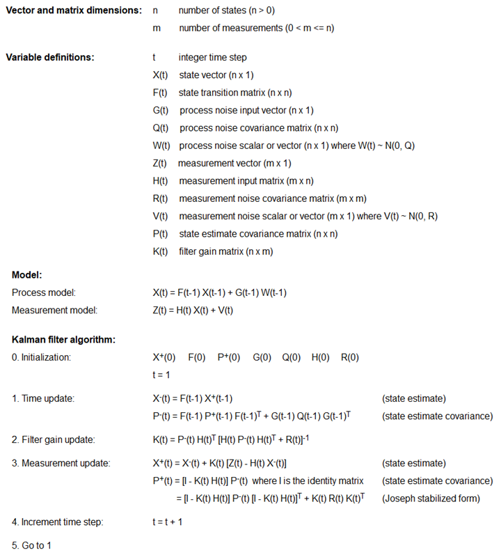
Standard Kalman filter process and measurement model equations, variable initialization, and algorithm steps are shown in Appendix 1. Since processes can contain multiple input, output, and state variables, Kalman filter equations are usually stated in matrix form, employing the operations of matrix addition, subtraction, multiplication, transposition (indicated by T), and inversion (indicated by -1). In the general case, all scalars, vectors, and matrices can potentially be time-varying (indicated by (t)).
The process model consists of:
- a vector X of the state variables,
- an additive process noise vector W ~ N(0, Q) where Q is the covariance of the process noise,
- a process noise input vector G which represents the effects of the process noise vector W at the previous integer time step t-1 on the state vector X at time step t, and
- a state transition matrix F representing a linear model of the process which translates the state vector X at the previous time step t-1 to time step t.
The process model equation shown in Appendix 1 does not include an external process control input term, since it is not relevant in the examples in this article.
The measurement model consists of:
- a measurement input matrix H which maps measurements of the state vector X to the measurement vector Z at time step t and
- an additive measurement noise vector V ~ N(0, R) where R is the covariance of the measurement noise.
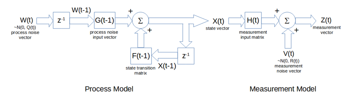
A matrix block diagram of the process and measurement models is shown below. The input to the process model is the process noise W(t), and the output is the state vector X(t). The inputs to the measurement model are the state vector X(t) and the measurement noise vector V(t), and the output is the measurement vector Z(t).
Each iteration of the Kalman filter algorithm at each time step t consists of three steps:
- The time update (also called the “predicted” or “a priori” update) of the state estimate vector, denoted by X–(t), and of the state estimate covariance matrix, denoted by P–(t) – The time update X–(t) projects, from the previous state measurement update X+(t-1), the effect of the process between time measurements, as modeled by the state transition matrix F(t-1). Similarly, the covariance time update P–(t) projects, from the previous covariance measurement update P+(t-1), the effect of the process between time measurements, as modeled by the transition matrix F(t-1), in addition to the effect of the previous process noise covariance Q(t-1), based on the process noise input vector G(t-1).
- The filter gain update of the gain matrix K(t) – The gain matrix K(t) determines the relative weighting used in the subsequent measurement update calculations, based on the relative uncertainties (as indicated by the covariances) of the current state time update P–(t) versus the current measurement noise R(t). More weight is given to the one with the lower uncertainty (smaller covariance). For example, if P–(t) is greater than R(t), the gain in the measurement update will give more weight to the latest measurement Z(t) than to the most recent state estimate X–(t). The filter gains range between 0 and 1.
- The measurement update (also called the “corrected” or “a posteriori” update) of the state estimate vector, denoted by X+(t), and of the state estimate covariance matrix, denoted by P+(t) – The measurement update X+(t) calculates a weighted sum of the most recent state estimate X–(t) and the latest measurement Z(t) based on the filter gain K(t). It also updates the covariance P+(t) from the time update P–(t) based on the filter gain. Note that, in addition to the standard form of the covariance measurement update P+(t) equation, the Joseph stabilized form, which is less sensitive to computer roundoff errors that can occur and accumulate over multiple iterations of the algorithm, is also shown and is the form used in the examples.
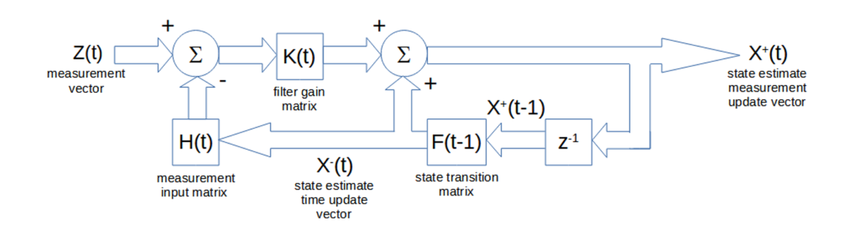
A matrix block diagram of the state estimate time update X–(t) and measurement update X+(t) calculations is shown below. The input is the measurement vector Z(t), and the output is the state estimate measurement update vector X+(t).
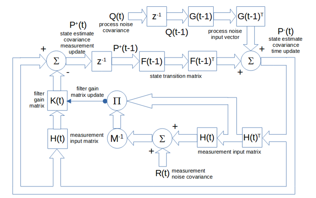
A matrix block diagram of the state estimate covariance time update P–(t) and standard (non-Joseph stabilized) measurement update P+(t) calculations and of the filter gain update K(t) calculations is shown below. The inputs are the process noise covariance Q(t) and the measurement noise covariance R(t). The internal output is the update of the elements of the gain matrix K(t).
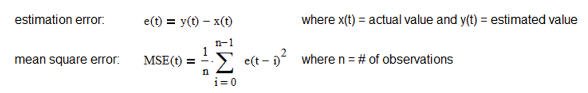
If the process and measurement models are linear and the process and measurement noise covariances are Gaussian, the Kalman filter is the optimal minimum mean square error (MSE) estimator. MSE is the average squared difference between the estimated values and the actual values over a sample of observations and is a statistical measure of the quality of the estimator – the smaller the MSE the better.
If the process and measurement models are linear but the process and measurement noise covariances are not Gaussian, the Kalman filter is the best linear estimator in the MSE sense. Non-linear models can be addressed using the extended Kalman filter or the unscented Kalman filter.
The Kalman filter assumes that the process and measurement noise covariances are known with some accuracy. Inaccurate noise covariance estimates can result in suboptimal state estimates and, in extreme cases, cause filter instability. The Kalman filter algorithm is also sensitive to inaccurate state variable initialization. In practice, the noise covariances, in particular, are often unknown or known only approximately. As a result, the most challenging aspect of Kalman filtering can be estimating the noise covariances.
3. Adaptive Kalman Filtering
There are two general types of Kalman filter models:
- steady-state models with fixed, time-invariant F, G, and H matrices that assume the process and measurement noise covariances are constant over time, resulting in fixed, time-invariant filter gains, and
- adaptive models with either fixed or time-varying F, G, and H matrices that assume the process and measurement noise covariances are not constant over time, resulting in time-varying filter gains.
A steady-state model will treat a shift in the process and measurement dynamics as a random effect, but, if the change is permanent, the filter may produce suboptimal state estimates as a result. Adaptive models, on the other hand, which are the focus of this article and Part 5, are able to adjust to processes that have time-varying dynamics, such as financial time series.
Several different types of adaptive Kalman filter methods have been proposed (6) (7), including:
- Bayesian estimation,
- maximum likelihood estimation,
- correlation methods,
- covariance matching, and
- multiple model filter banks.
Some of these methods can be complex to implement and do not always respond rapidly enough to the volatility and non-stationarity of financial time series to be useful for trading purposes. The next section describes an adaptive covariance matching method that uses noise samples generated directly from the Kalman filter algorithm, replacing, for example, the need for assumed or externally-derived noise covariance estimates.
4. One State Noise-Adaptive Kalman Filter
The noise-adaptive method described here was originally proposed by Myers and Tapley (8) and re-stated with some modification by Stengel (9). The Stengel version is used in this article and in Part 5. The method estimates the process and measurement noise covariances simultaneously with the state estimates.
In part to more easily illustrate the adaptive filter concepts and calculations, a one-state Kalman filter is used in the examples in this article. The one-state Kalman filter is based on a first-order process model that has a locally constant mean value a contaminated by additive random noise ε(t) ~ N(0, σε2):
y(t) = a + ε(t)
More specifically, the process models in both articles are based on the assumption that financial asset prices follow the general Newtonian equation of motion (10):
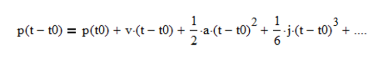
where p is the position (analogous to a financial asset price), v is the velocity (analogous to what is commonly called “momentum” by quantitative analysts and market technicians), a is the acceleration (change in velocity), j is the jerk (change in acceleration), etc.
In the case of the one-state Kalman filter, the state variable scalar x(t) is equivalent to first-order process model mean value a as well as to Newtonian position p (i.e., velocity v = 0, acceleration a = 0, jerk j = 0, etc.). Part 5 illustrates a two-stage Kalman filter, based on a second-order process model that has a mean value a and linear trend b contaminated by additive random noise. The two-state variables are equivalent to Newtonian position p and velocity v.
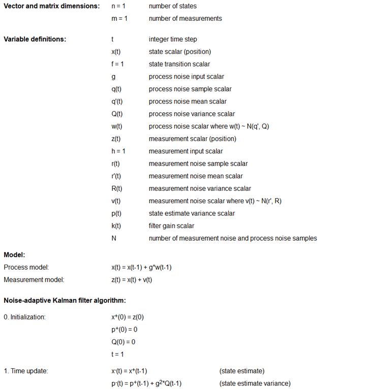
The one-state noise-adaptive Kalman filter process and measurement model equations, variable initialization, algorithm steps, and noise estimate calculations are shown in Appendix 2 where:
- the number of state variables n = 1,
- the state position variable x(t) is a scalar,
- the number of measurements m = 1 since only position (i.e., price) measurements z(t) are available,
- the time step is 1 trading day,
- the state transition scalar f = 1 since the Newtonian motion equation that includes only position p is p(t) = p(t-1),
- the process noise input scalar g = 1, based on the process model assumption that the position is locally constant and subject to random velocity noise,
- the process noise variance Q(t) is a scalar,
- the state measurement input scalar h = 1 since only position is measured,
- the filter gain scalar k(t) ranges between 0 and 1, and
- the number of process and measurement noise samples N in the sliding time window is 10 trading days.
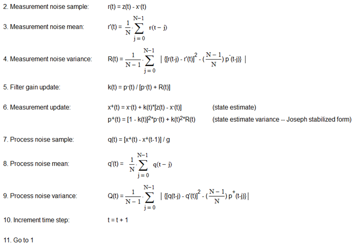
Since only measurements z(t) of position are available in the one state filter, the noise-adaptive method uses a set of measurement noise samples r(t), also called “residuals”, where:
r(t) = z(t) – x–(t)
made over a sliding time window of length N time steps (N > 1) to estimate the measurement noise mean r’(t) and variance R(t). That is, the most recent set of N noise samples made over time steps t-N+1 to t is used in the calculations at each time step t. It uses a set of approximate position process noise samples q(t) where:
q(t) = [x+(t) – x+(t-1)] / g
and g is the position process noise input scalar, made over the sliding time window to estimate the process noise mean q’(t) and variance Q(t). The measurement and process noise means and variances are re-estimated each time the window is shifted forward by a one-time step.
A block diagram of the measurement noise variance R(t) and process noise variance Q(t) estimate calculations for the one-state noise-adaptive Kalman filter is shown below.
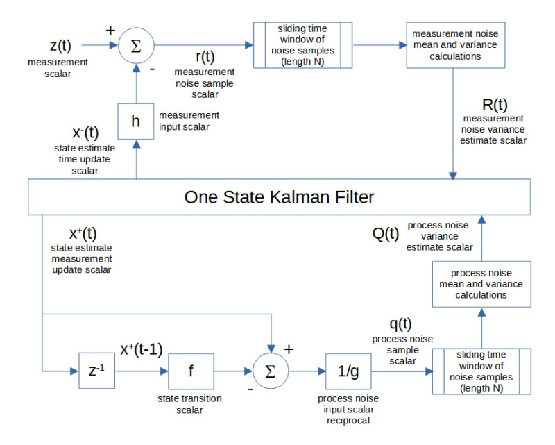
Notes:
- Because the measurement noise variance R(t) and process noise variance Q(t) may in actual practice become negative when performing the estimate calculations, the absolute values of the summation terms are used (11).
- In order to minimize potential problems in the initialization process, an expanding time window, i.e., including noise samples at time steps 1 to t, is used to calculate the process noise and measurement noise mean and variance estimates for time steps 1 through N-1, after which the sliding time window of length N is used.
- In order to minimize potential roundoff errors, the Joseph stabilized form of the state estimate variance measurement update p+(t) equation is used.
5. One State Noise-Adaptive Kalman Filter Examples
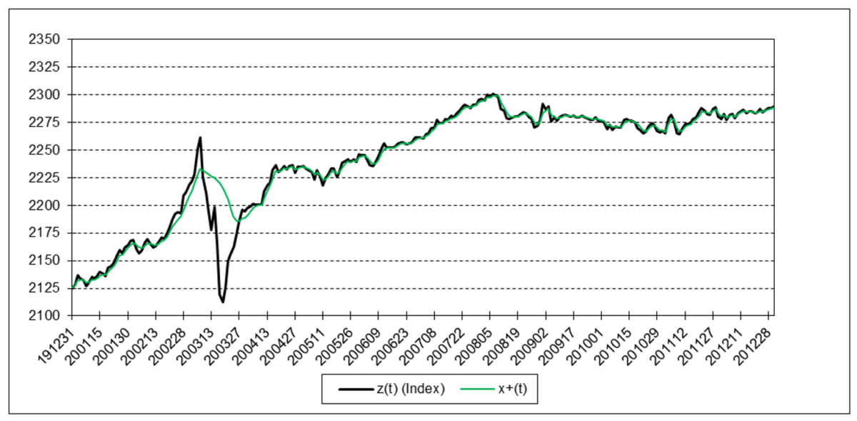
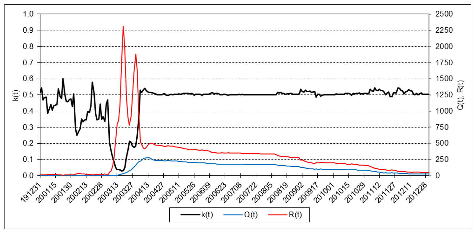
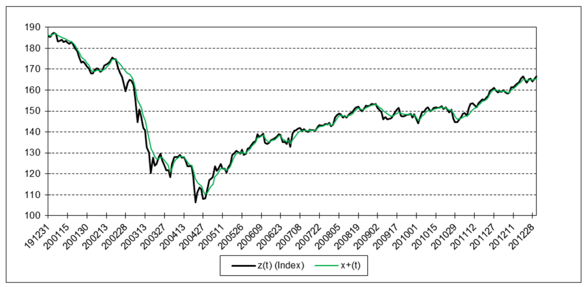
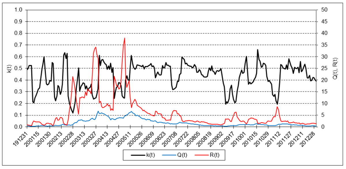
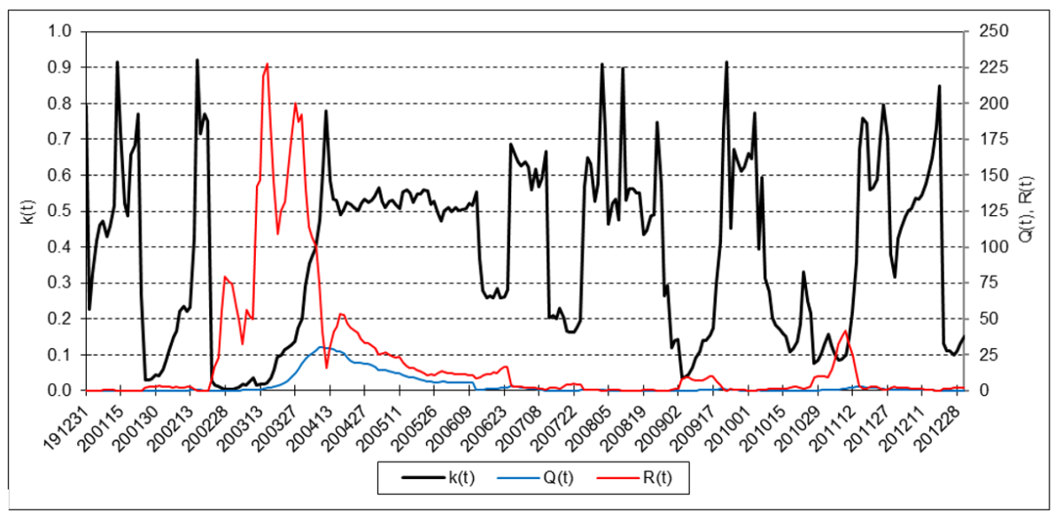
The following charts illustrate the application of the one-state noise-adaptive Kalman filter method to the daily closing values of a stock index, a bond index, a currency, a commodity index, and a volatility index for the year 2020. The upper chart of each example shows the index or FX rate input z(t) and the state estimate measurement update output x+(t). The lower chart shows the filter gain k(t) and associated Q(t) and R(t) variances.
S&P 500 Stock Index
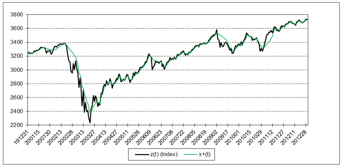
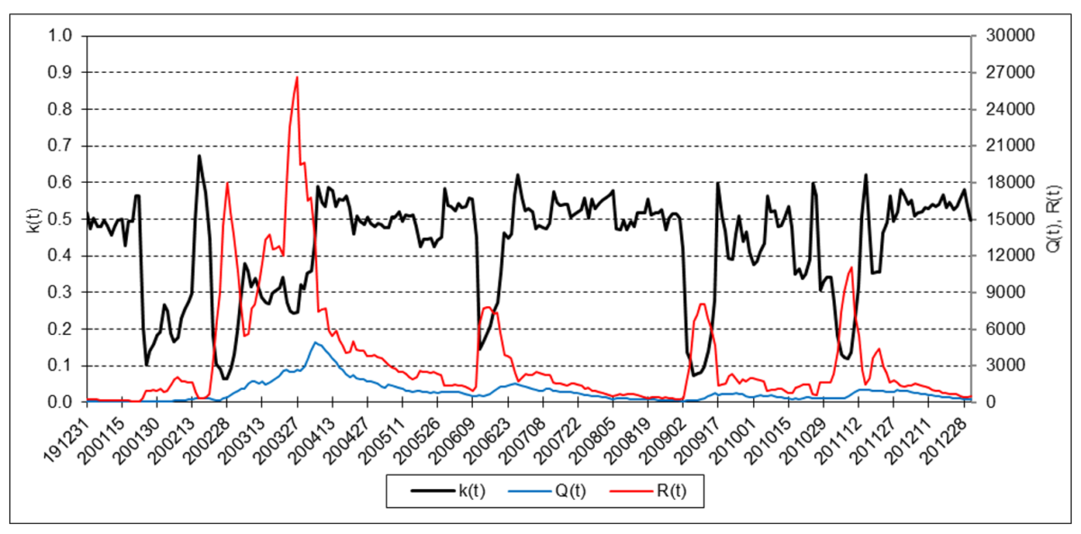
The results are hypothetical results and are NOT an indicator of future results and do NOT represent returns that any investor actually attained. Indexes are unmanaged, do not reflect management or trading fees, and one cannot invest directly in an index.
Bloomberg U.S. Aggregate Bond Index
The results are hypothetical results and are NOT an indicator of future results and do NOT represent returns that any investor actually attained. Indexes are unmanaged, do not reflect management or trading fees, and one cannot invest directly in an index.
Euro
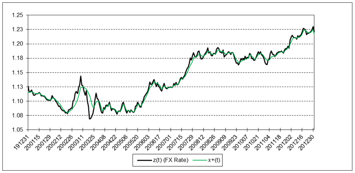
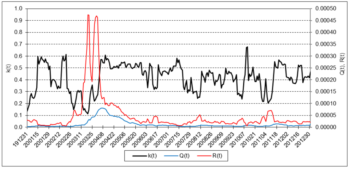
The results are hypothetical results and are NOT an indicator of future results and do NOT represent returns that any investor actually attained. Indexes are unmanaged, do not reflect management or trading fees, and one cannot invest directly in an index.
Refinitiv/CoreCommodity CRB Index
The results are hypothetical results and are NOT an indicator of future results and do NOT represent returns that any investor actually attained. Indexes are unmanaged, do not reflect management or trading fees, and one cannot invest directly in an index.
Cboe Volatility Index (VIX)
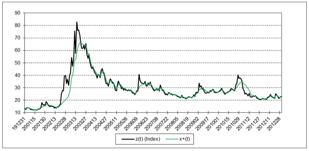
The results are hypothetical results and are NOT an indicator of future results and do NOT represent returns that any investor actually attained. Indexes are unmanaged, do not reflect management or trading fees, and one cannot invest directly in an index.
6. Trading Signal Generation
A trading signal using the one state noise-adaptive Kalman filter can potentially be generated, for example, when the position measurement z(t) crosses above (buy) or below (sell) the position state estimate, x+(t).
7. Comments
The one-state noise-adaptive Kalman filter output response can be modified by adjusting the length N of the sliding time window. The smaller N, the more responsive the filter is to changing process and measurement noise dynamics.
The utility of a one-state Kalman filter may be limited due to the fact that the filter is modeled on a first-order process. If the measurement input z(t) contains linear or higher-order trends (i.e., non-zero velocity v, acceleration a, jerk j, etc.), a one-state Kalman filter output will lag the input because the filter is not designed to model trends.
The Kalman filter algorithm assumes that the process and measurement noise covariance probability distributions are normal. The noise-adaptive mean and variance estimate calculations also assume normality. Since financial time series are typically observed to be non-normal(12), the filter may produce suboptimal state estimates. Other estimation methods, such as the particle filter, do not assume normality.
8. Side Note on the One State Steady-State Kalman Filter
A one-state steady-state Kalman filter where the state transition scalar f = 1, the measurement input scalar h = 1, the process noise input scalar g is time-invariant, and the Q and R noise variances are constant is closely related to the alpha tracking filter, single exponential smoothing, and the ARIMA(0,1,1) time series model (13) (14).
If either Q and R or the Q/R ratio is known, if initialized to an arbitrary value, the filter gain k will converge to a steady-state value that can be calculated directly. The equation for k as a function of Q/R and g is:
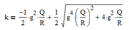
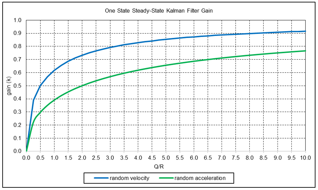
The graph below shows k as a function of Q/R for the random velocity noise process model (g = 1) and also for the process model based on the assumption that the position is locally constant and subject to random acceleration noise (g = ½)(15). In both cases, the filter gain increases as Q/R increases.
The general solution approach to derive steady-state Kalman filter gains is described in Appendix 3.
Acknowledgements
I would like to thank Larry Stabile for reviewing this article and providing many helpful comments and suggestions.
Appendix 1 – Kalman Filter
Appendix 2 – One State Noise-Adaptive Kalman Filter
Appendix 3 – Steady-State Kalman Filter Gain Derivation
The general solution approach to derive the steady-state Kalman filter gain K where the F, G, and H matrices are time-invariant and the Q and R noise covariances are constant assumes that the state estimate covariance time update:
P– = F P+ FT + G Q GT (1)
and the state estimate covariance measurement update:
P+ = [I – K H] P– (2)
where I is the identity matrix, are equal in steady state, i.e., P– = P + (16). Solving (2) for P– gives:
P– = P+ [I – K H]-1 (3)
Setting (1) and (3) equal gives:
F P+ FT + G Q GT = P+ [I – K H]-1 (4)
An alternate form of the Kalman filter gain update equation is:
K = P+ HT R-1 (5)
Solving (5) for P+ gives:
P+ = K R (HT)-1 (6)
Substituting (6) for P+ in (4) gives:
F K R (HT)-1 FT + G Q GT = K R (HT)-1 [I – K H]-1 (7)
Solving (7) for K results in the following equation:

References[+]
| ↑1 | See for example: Gelb, A., ed., Applied Optimal Estimation, The M.I.T. Press, 1974; Brown, R. G. and Hwang, P. Y. C., Introduction to Random Signals and Applied Kalman Filtering, John Wiley & Sons, Inc., 2012; and KalmanFilter.NET (https://www.kalmanfilter.net). |
|---|---|
| ↑2 | Kalman, R. E., “A New Approach to Linear Filtering and Prediction Problems”, Journal of Basic Engineering, 82 (1), 35-45, March 1960. |
| ↑3 | Swerling, P., “First-Order Error Propagation in a Stagewise Smoothing Procedure for Satellite Observations”, U.S. Air Force Project RAND Research Memorandum RM-2329, The RAND Corporation, June 15, 1959 |
| ↑4 | Stratonovich, R. L., “Optimum Nonlinear Systems Which Bring About a Separation of a Signal with Constant Parameters from Noise”, Radiofizika, 2 (6), 892-901, 1959. |
| ↑5 | Kalman, R. E., and Bucy, R. S, “New Results in Linear Filtering and Prediction Theory”, Journal of Basic Engineering, 83 (1), 95-108, March 1961. |
| ↑6 | Mehra, R. E., “Approaches to Adaptive Filtering”, IEEE Transactions on Automatic Control, AC-17 (5), 693-698, October 1972. |
| ↑7 | Alspach, D. L., “A Parallel Filtering Algorithm for Linear Systems with Unknown Time-Varying Noise”, IEEE Transactions on Automatic Control, AC-19 (5), 552-556, October 1974. |
| ↑8 | Myers, K. A. and Tapley, B. D., “Adaptive Sequential Estimation with Unknown Noise Statistics”, IEEE Transactions on Automatic Control, AC-21 (4), 520-523, August 1976. |
| ↑9 | Stengel, R. F., Optimal Control and Estimation, Dover Publications, Inc., 1994. |
| ↑10 | Lopez de Prado, M. and Rebonato, R., “Kinetic Component Analysis”, Journal of Investing, 25 (3), 142-154, Fall 2016. |
| ↑11 | Myers, K. A. and Tapley, B. D., “Adaptive Sequential Estimation with Unknown Noise Statistics”, IEEE Transactions on Automatic Control, AC-21 (4), 520-523, August 1976 |
| ↑12 | ”An Introduction to Digital Signal Processing for Trend Following“ |
| ↑13 | Kalata, P. R., “The Tracking Index: A Generalized Parameter for α-β and α-β-γ Target Trackers”, IEEE Transactions on Aerospace and Electronic Systems, AES-20 (2), 174-182, March 1984. |
| ↑14 | Abraham, B. and Ledolter, J., “Forecast Functions Implied by Autoregressive Integrated Moving Average Models and Other Related Forecast Procedures”, International Statistical Review, 54 (1), 51-66, April 1986. |
| ↑15 | Kalata, P. R., “The Tracking Index: A Generalized Parameter for α-β and α-β-γ Target Trackers”, IEEE Transactions on Aerospace and Electronic Systems, AES-20 (2), 174-182, March 1984. |
| ↑16 | Blair, W. D., “Fixed Gain, Two Stage Estimators for Tracking Maneuvering Targets”, Naval Surface Warfare Center, Dahlgren Division, NSWCDD/TR-92/297, July 1992. |
About the Author: Henry Stern
—
Important Disclosures
For informational and educational purposes only and should not be construed as specific investment, accounting, legal, or tax advice. Certain information is deemed to be reliable, but its accuracy and completeness cannot be guaranteed. Third party information may become outdated or otherwise superseded without notice. Neither the Securities and Exchange Commission (SEC) nor any other federal or state agency has approved, determined the accuracy, or confirmed the adequacy of this article.
The views and opinions expressed herein are those of the author and do not necessarily reflect the views of Alpha Architect, its affiliates or its employees. Our full disclosures are available here. Definitions of common statistics used in our analysis are available here (towards the bottom).
Join thousands of other readers and subscribe to our blog.