1. Introduction
Previous articles in this series examine, from a digital signal processing (DSP) frequency domain perspective, various types of digital filters used by quantitative analysts and market technicians to analyze and transform financial time series for trend-following purposes.
- An Introduction to Digital Signal Processing for Trend Following
- Trend-Following Filters – Part 1
- Trend-Following Filters – Part 2
- Trend-Following Filters – Part 3
- Trend-Following Filters – Part 4
Part 4 of this series, along with this article, examines the application of the Kalman filter to financial time series. The Kalman filter is a statistics-based algorithm used to perform estimation of random processes(1). Estimation of processes in noisy environments is a critical task in many fields, such as communications, process control, track-while-scan radar systems, robotics, and aeronautical, missile, and space vehicle guidance. The Kalman filter is a real-time algorithm that operates iteratively in the discrete-time domain and is used in a variety of complex random process estimation applications.
There are two general types of Kalman filter models: steady-state and adaptive. A steady-state filter assumes that the statistics of the process under consideration are constant over time, resulting in fixed, time-invariant filter gains. The gains of an adaptive filter, on the other hand, are able to adjust to processes that have time-varying dynamics, such as financial time series which typically display volatility and non-stationarity.
2. Two State Noise-Adaptive Kalman Filter
This article assumes familiarity with Part 4, which includes an overview of the Kalman filter and describes an adaptive covariance matching method originally proposed by Myers and Tapley (2) and re-stated with some modification by Stengel (3). The Stengel version is employed in both articles. The method estimates the process and measurement noise covariances directly from the Kalman filter algorithm, replacing, for example, the need for assumed or externally-derived noise covariance estimates.
To more easily illustrate adaptive filter concepts and calculations, the Kalman filter algorithm described in Part 4 has one state variable, x(t), modeled on a first-order process that has a locally constant mean value a contaminated by additive random noise ε(t)~N(0, σε2):
y(t) = a + ε(t)
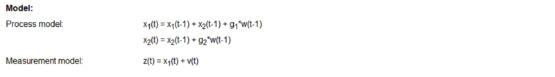
The filter described in this article has two state variables, x1(t) and x2(t), modeled on a second-order process that has mean value a and locally constant linear trend b contaminated by additive random noise:
y(t) = a + b*t + ε(t)
More specifically, the process models in both articles are based on the assumption that financial asset prices follow the general Newtonian equation of motion (4):

where p is the position (analogous to a financial asset price), v is the velocity (analogous to what is commonly called “momentum” by quantitative analysts and market technicians), a is the acceleration (change in velocity), j is the jerk (change in acceleration), etc. State variable x1(t) is equivalent to the second-order process mean value a as well as to Newtonian position p. State variable x2(t) is equivalent to second-order process linear trend b as well as to Newtonian velocity v (i.e., it is assumed that acceleration a = 0, jerk j = 0, etc.).
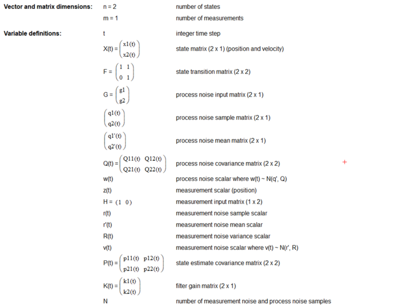
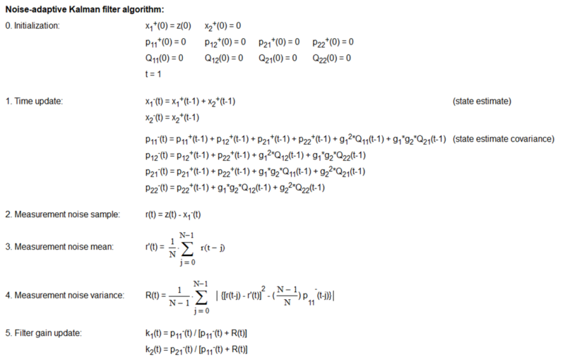
The two-state noise-adaptive Kalman filter process and measurement model equations, variable initialization, algorithm steps, and noise estimate calculations are shown in Appendix 1 where:
- the number of state variables n = 2,
- the two state variables are position x1(t) and velocity x2(t),
- the number of measurements m = 1 since only position (i.e., price) measurements z(t) are assumed to be available,
- the time step is 1 trading day,
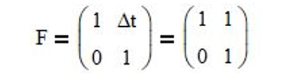
- since the Newtonian motion equations that include only position p and velocity v are p(t) = p(t-1) + v*Δt and v(t) = v(t-1), respectively, the state transition matrix is:
- the process noise inputs g1 = ½ and g2 = 1, based on the process model assumption that the velocity is locally constant and subject to random acceleration noise (5),
- the state measurement input vector H = (1 0) since only position is measured,
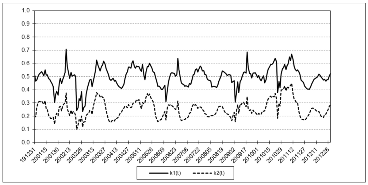
- the filter gains k1(t) and k2(t) range between 0 and 1, and
- the number of process and measurement noise samples N in the sliding time window is 10 trading days.
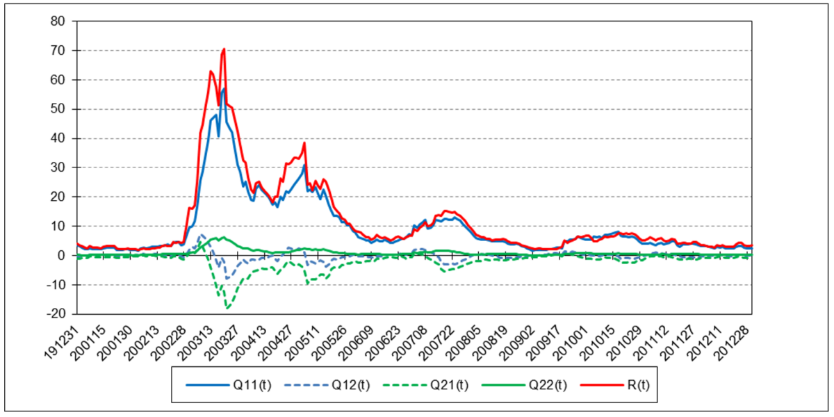
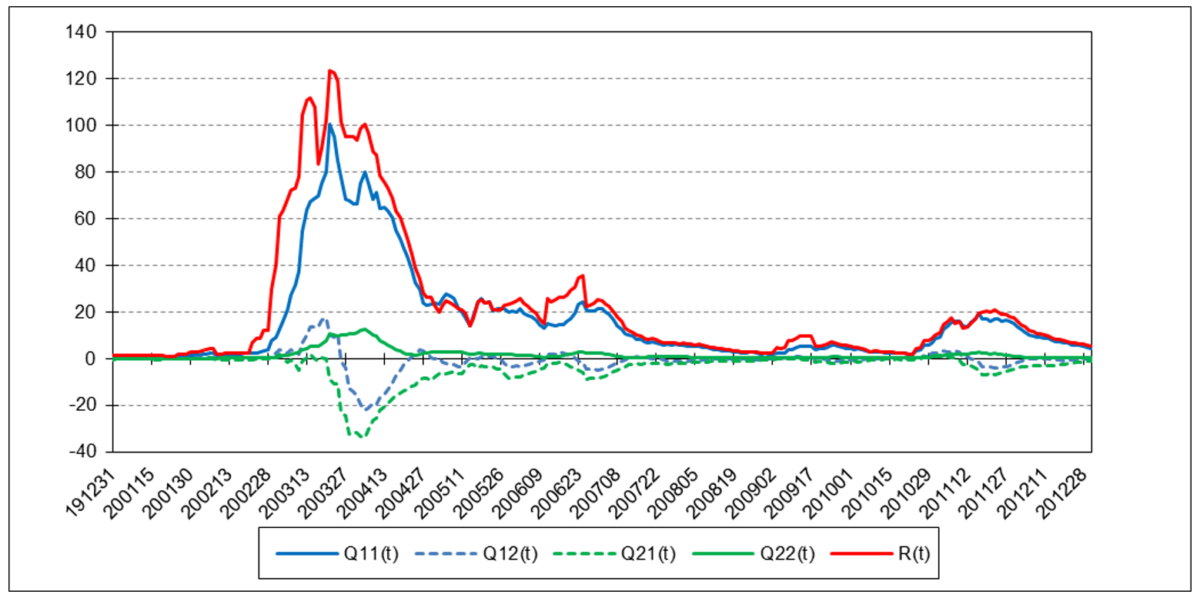
The noise-adaptive method estimates the measurement and process noise covariances simultaneously with the state estimates. Since only measurements z(t) of position are available, the noise-adaptive method uses a set of measurement noise samples r(t), also called “residuals”, where:
r(t) = z(t) – x1–(t)
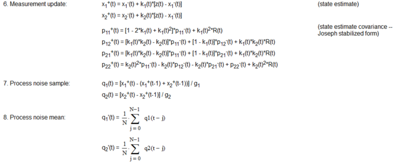
made over a sliding time window of length N time steps (N > 1) to estimate the measurement noise mean r’(t) and variance R(t). That is, the most recent set of N noise samples made over time steps t-N+1 to t is used in the calculations at each time step t. It uses sets of approximate position and velocity process noise samples q1(t) and q2(t), respectively, where:
q1(t) = [x1+(t) – (x1+(t-1) + x2+(t-1))] / g1
q2(t) = [x2+(t) – x2+(t-1)] / g2
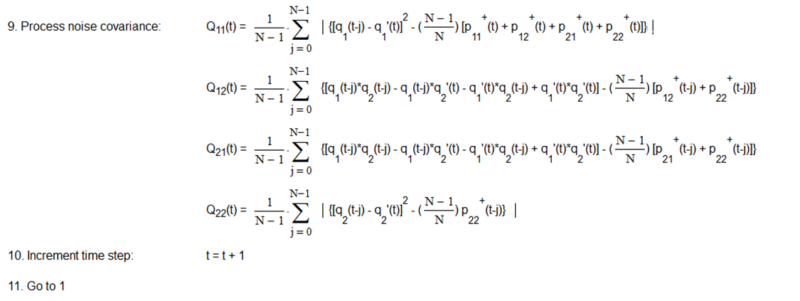
and g1 and g2 are the position and velocity process noise input scalars, respectively, made over the sliding time window to estimate the process noise means q1’(t) and q2’(t) and covariances Q11(t), Q12(t), Q21(t), and Q22(t). The measurement and process noise means and covariances are re-estimated each time the window is shifted forward by one time step.
Notes:
- The filter equations in Appendix 1 are shown in non-matrix form for clarity.
- Because the measurement noise variance R(t) and process noise covariance Q(t) may in actual practice become negative definite when performing the estimate calculations, the absolute values of the summation terms of R(t), Q11(t), and Q22(t) are used (6).
- In order to minimize potential problems in the initialization process, an expanding time window, i.e., including noise samples at time steps 1 to t, is used to calculate the process noise and measurement noise mean and covariance estimates for time steps 1 through N-1, after which the sliding time window of length N is used.
- In order to minimize potential roundoff errors, the Joseph stabilized form of the state estimate covariance measurement update P+(t) equations is used.
3. Two State Noise-Adaptive Kalman Filter Examples
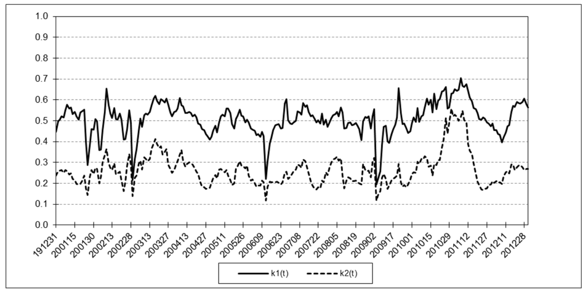
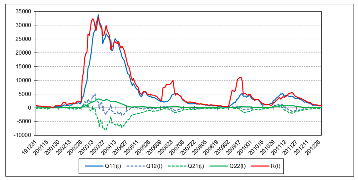
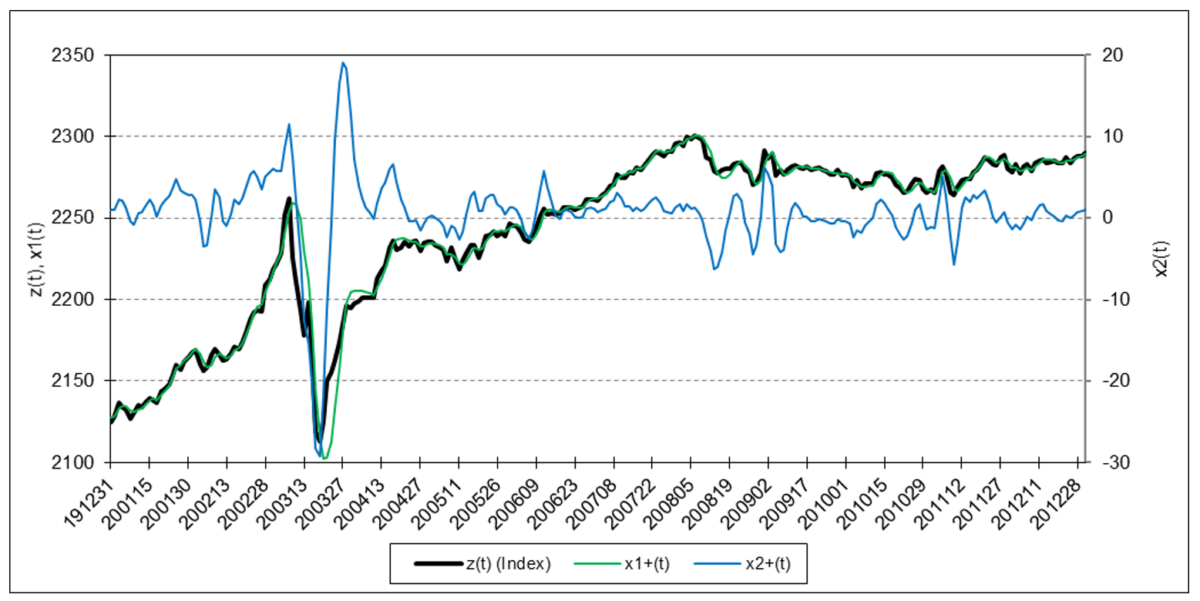
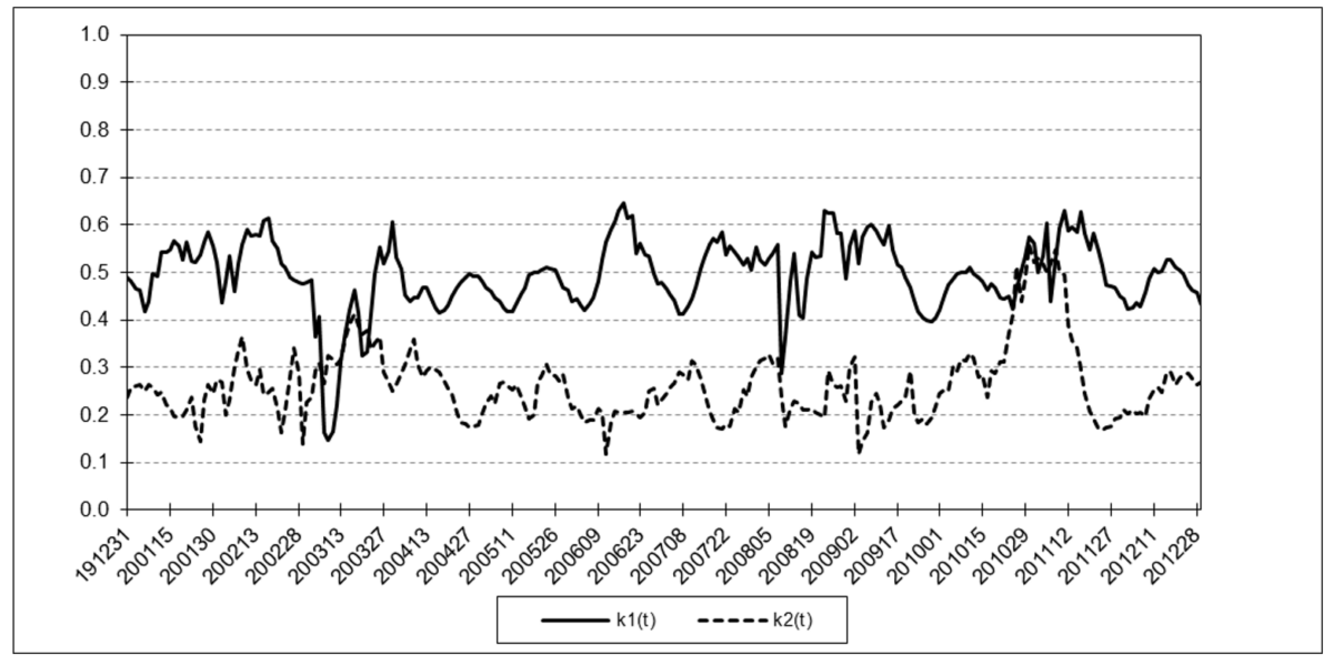
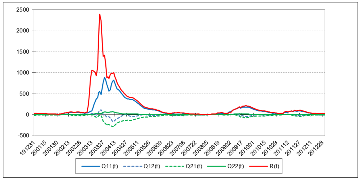
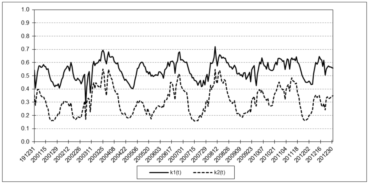
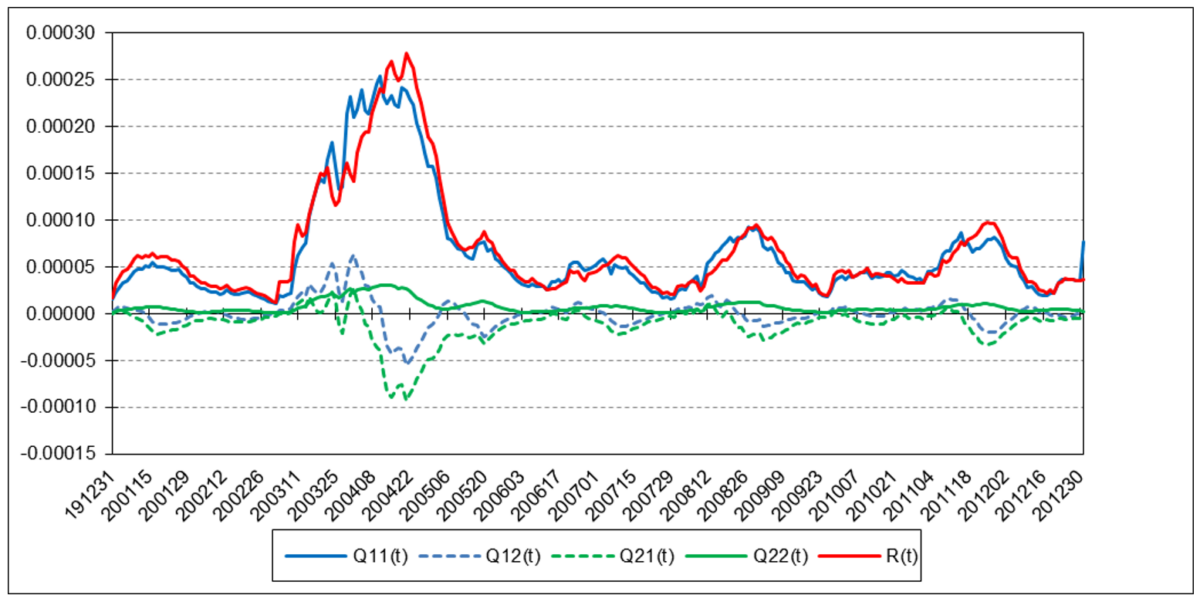
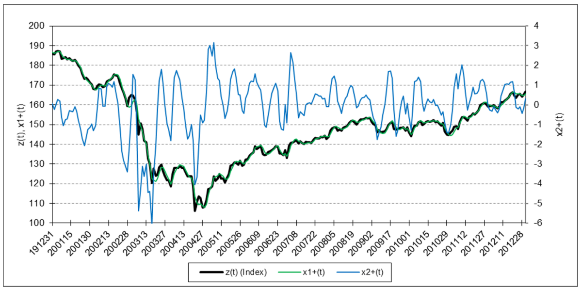
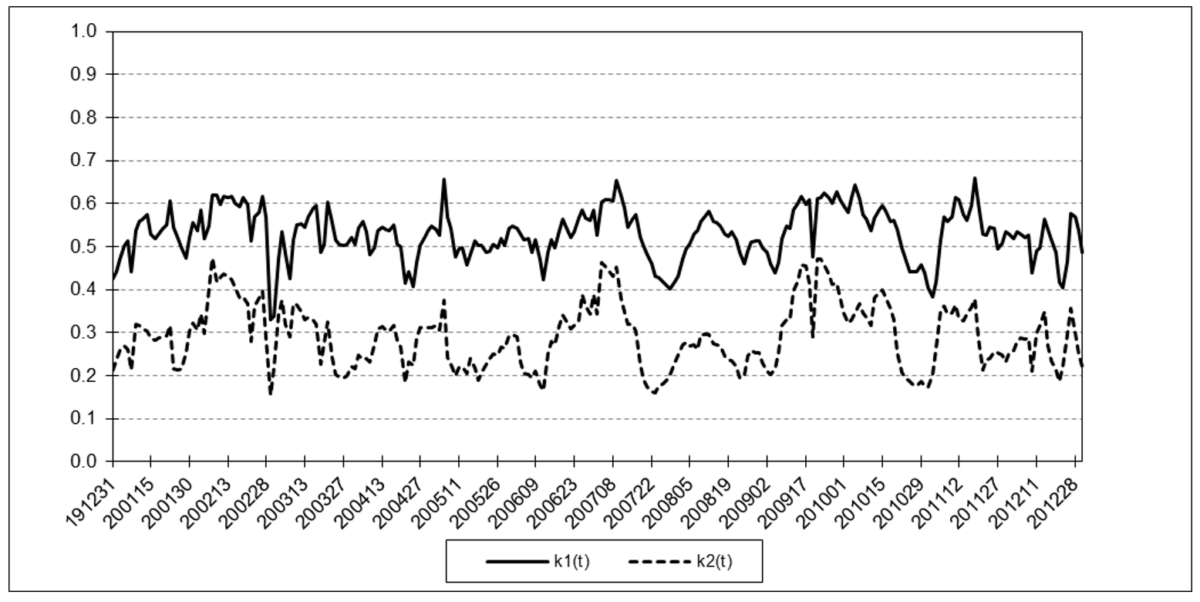
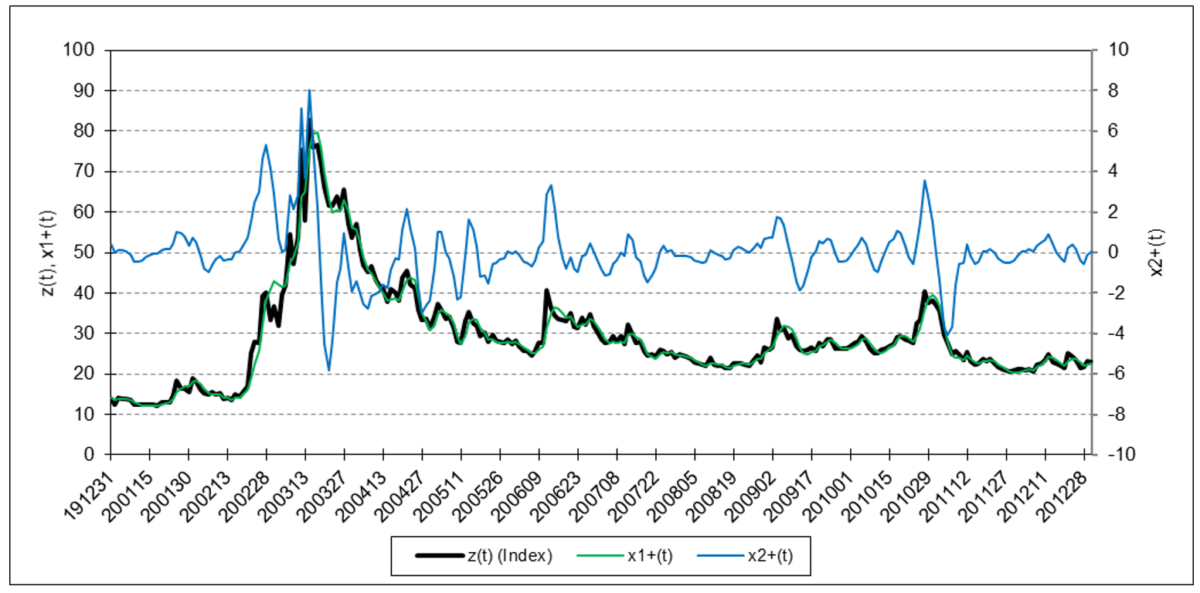
The following charts illustrate the application of the two-state noise-adaptive Kalman filter method to the daily closing values of a stock index, a bond index, a currency, a commodity index, and a volatility index for the year 2020. The upper chart of each example shows the index or FX rate input z(t) and the state estimate measurement update outputs x1+(t) and x2+(t), the middle chart shows the filter gains k1(t) and k2(t), and the lower chart shows the associated Q(t) and R(t) covariances.
S&P 500 Stock Index
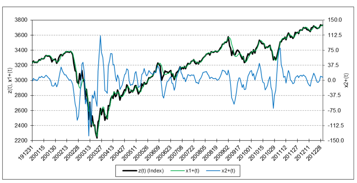
The results are hypothetical results and are NOT an indicator of future results and do NOT represent returns that any investor actually attained. Indexes are unmanaged, do not reflect management or trading fees, and one cannot invest directly in an index.
Bloomberg U.S. Aggregate Bond Index
The results are hypothetical results and are NOT an indicator of future results and do NOT represent returns that any investor actually attained. Indexes are unmanaged, do not reflect management or trading fees, and one cannot invest directly in an index.
Euro
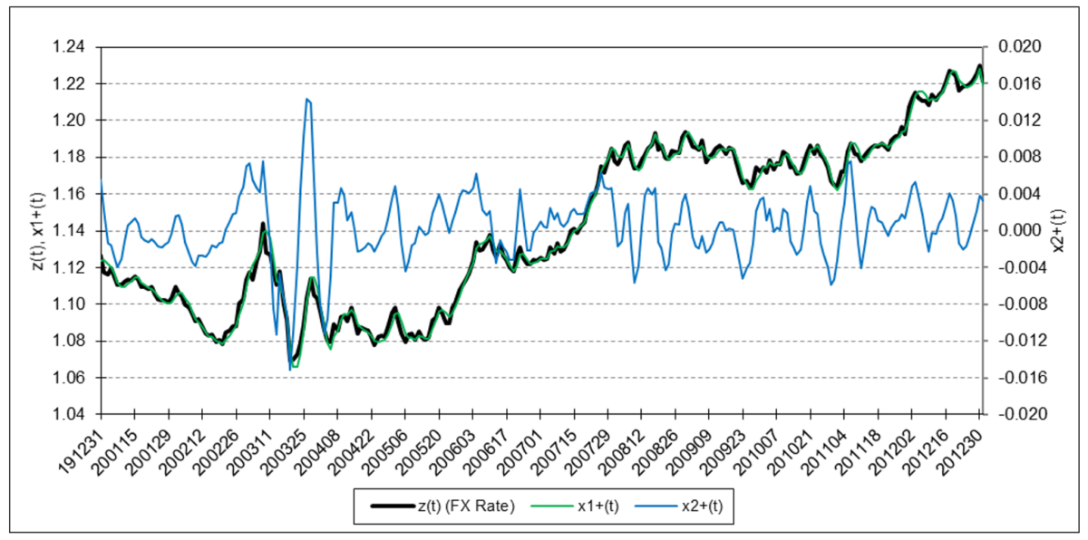
The results are hypothetical results and are NOT an indicator of future results and do NOT represent returns that any investor actually attained. Indexes are unmanaged, do not reflect management or trading fees, and one cannot invest directly in an index.
Refinitiv/CoreCommodity CRB Index
The results are hypothetical results and are NOT an indicator of future results and do NOT represent returns that any investor actually attained. Indexes are unmanaged, do not reflect management or trading fees, and one cannot invest directly in an index.
Cboe Volatility Index (VIX)
The results are hypothetical results and are NOT an indicator of future results and do NOT represent returns that any investor actually attained. Indexes are unmanaged, do not reflect management or trading fees, and one cannot invest directly in an index.
4. Trading Signal Generation
Trading signals using the two-state noise-adaptive Kalman filter can potentially be generated, for example, when:
- the position measurement z(t) crosses above (buy) or below (sell) the position state estimate x1+(t),
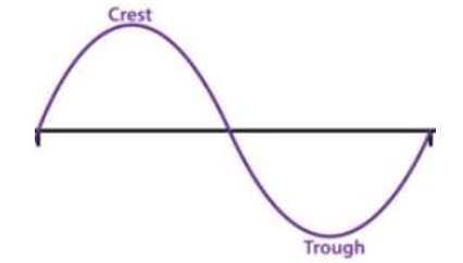
- the position state estimate x1+(t) reaches a local crest (sell) or trough (buy),
- the velocity state estimate x2+(t) crosses above (buy) or below (sell) the zero line,
- the velocity state estimate x2+(t) reaches a local crest (sell) or trough (buy),
or by a combination of these conditions.
5. Comments
The two-state noise-adaptive Kalman filter output response can be modified by adjusting the length N of the sliding time window. The smaller N, the more responsive the filter is to changing process and measurement noise dynamics.
The utility of a two-state Kalman filter may be limited due to the fact that the filter is modeled on a second-order process. If the measurement input z(t) contains quadratic or higher-order trends (i.e., non-zero acceleration a, jerk j, etc.), a two-state Kalman filter output will lag the input because the filter is not designed to model those types of trends.
Setting the two-state noise-adaptive Kalman filter process noise inputs g1 = 1 and g2 = 0, based on the process model assumption that the position is locally constant and subject to random velocity noise, generates essentially the same output as the one-state noise-adaptive Kalman filter illustrated in Part 4.
The Kalman filter algorithm assumes that the process model can be represented by a set of input, output, and state variables that are related by linear difference equations. Non-linear models can be addressed using the extended Kalman filter or the unscented Kalman filter.
The Kalman filter algorithm also assumes that the process and measurement noise covariance probability distributions are normal. The noise-adaptive mean and covariance estimate calculations also assume normality. Since financial time series are typically observed to be non-normal, the filter may produce suboptimal state estimates. Other estimation methods, such as the particle filter, do not assume normality.
6. Side Note on the Two-State Steady-State Kalman Filter
A two-state steady-state Kalman filter, where the state transition matrix F is Newtonian, the measurement input matrix H measures the position only, the process noise input matrix G is time-invariant, and the Q and R noise covariances are constant, is closely related to the alpha-beta tracking filter, Holt additive linear trend smoothing, and the ARIMA(0,2,2) time series model (7) (8).
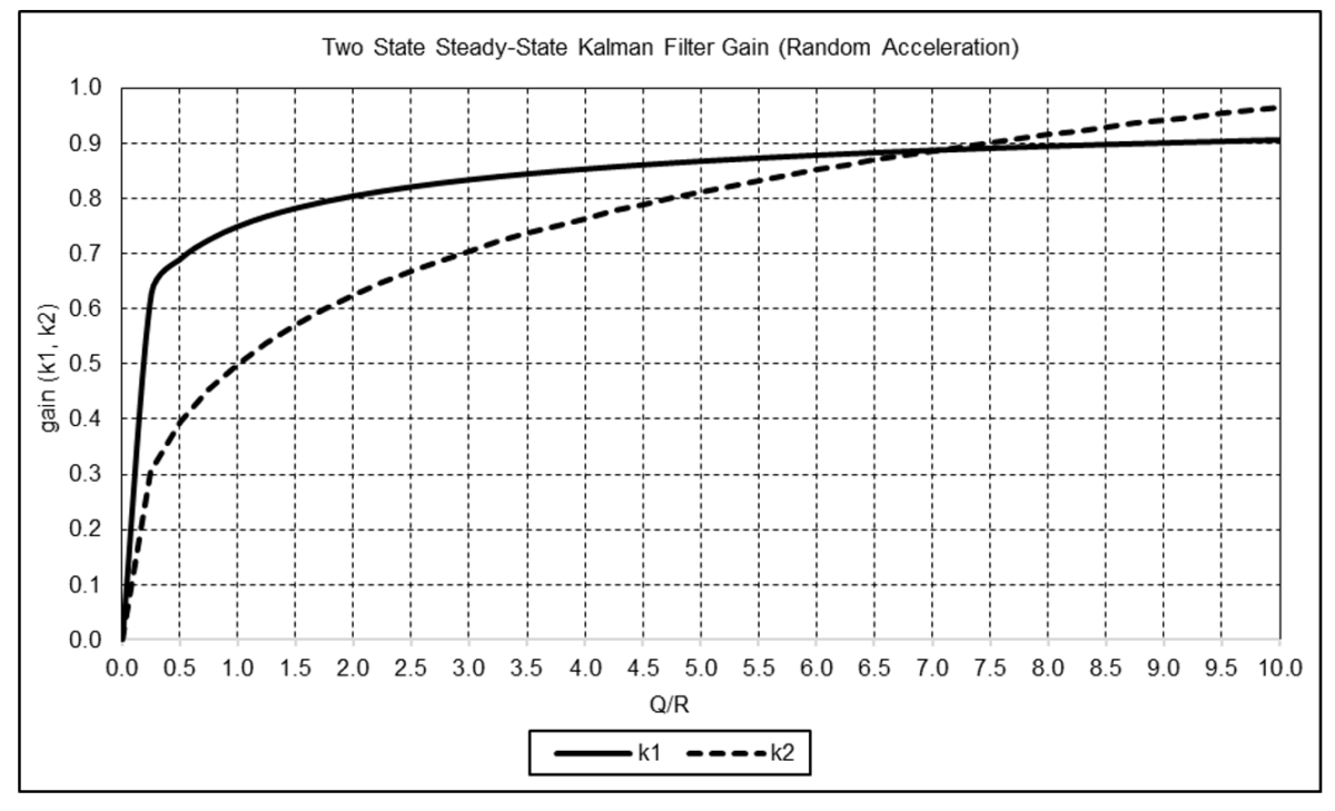
If either Q and R or the Q/R ratio is known, if initialized to arbitrary values, the filter gains k1 and k2 will converge to steady-state values that can be calculated directly. For the random acceleration noise model (g1 = ½ and g2 = 1), the equations are:
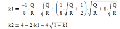
The graph below shows k1 and k2 as functions of Q/R for this model. The filter gains increase as Q/R increases.
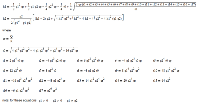
The general equations for the two-state steady-state Kalman filter gains k1 and k2 as functions of Q/R, g1, and g2 where the F matrix is Newtonian, the H matrix measures the position only, and the Q and R noise covariances are constant are shown in Appendix 2.
Acknowledgements
I would like to thank Larry Stabile for reviewing this article and providing many helpful comments and suggestions.
Appendix 1 – Two State Noise-Adaptive Kalman Filter
Appendix 2 – Two State Steady-State Kalman Filter Gains
The solution approach to derive steady-state Kalman filter gains is described in Appendix 3 of Part 4.
The equations for the two-state steady-state Kalman filter gains k1 and k2 as functions of Q/R, g1, and g2 where the F matrix is Newtonian, the H matrix measures the position only, and the Q and R noise covariances are constant are:
References[+]
| ↑1 | Kalman, R. E., “A New Approach to Linear Filtering and Prediction Problems”, Journal of Basic Engineering, 82 (1), 35-45, March 1960. |
|---|---|
| ↑2 | Myers, K. A. and Tapley, B. D., “Adaptive Sequential Estimation with Unknown Noise Statistics”, IEEE Transactions on Automatic Control, AC-21 (4), 520-523, August 1976. |
| ↑3 | Stengel, R. F., Optimal Control and Estimation, Dover Publications, Inc., 1994. |
| ↑4 | Lopez de Prado, M. and Rebonato, R., “Kinetic Component Analysis”, Journal of Investing, 25 (3), 142-154, Fall 2016. |
| ↑5 | Kalata, P. R., “The Tracking Index: A Generalized Parameter for α-β and α-β-γ Target Trackers”, IEEE Transactions on Aerospace and Electronic Systems, AES-20 (2), 174-182, March 1984. |
| ↑6 | Myers, K. A. and Tapley, B. D., “Adaptive Sequential Estimation with Unknown Noise Statistics”, IEEE Transactions on Automatic Control, AC-21 (4), 520-523, August 1976. |
| ↑7 | Kalata, P. R., “The Tracking Index: A Generalized Parameter for α-β and α-β-γ Target Trackers”, IEEE Transactions on Aerospace and Electronic Systems, AES-20 (2), 174-182, March 1984. |
| ↑8 | Abraham, B., and Ledolter, J., “Forecast Functions Implied by Autoregressive Integrated Moving Average Models and Other Related Forecast Procedures”, International Statistical Review, 54 (1), 51-66, April 1986. |
About the Author: Henry Stern
—
Important Disclosures
For informational and educational purposes only and should not be construed as specific investment, accounting, legal, or tax advice. Certain information is deemed to be reliable, but its accuracy and completeness cannot be guaranteed. Third party information may become outdated or otherwise superseded without notice. Neither the Securities and Exchange Commission (SEC) nor any other federal or state agency has approved, determined the accuracy, or confirmed the adequacy of this article.
The views and opinions expressed herein are those of the author and do not necessarily reflect the views of Alpha Architect, its affiliates or its employees. Our full disclosures are available here. Definitions of common statistics used in our analysis are available here (towards the bottom).
Join thousands of other readers and subscribe to our blog.