Machine Learning for Investors: A Primer

If you are out to describe the truth, leave elegance to the tailor.

— Albert Einstein

Machine learning is everywhere now, from self-driving cars to Siri and Google Translate, to news recommendation systems and, of course, trading.

In the investing world, machine learning is at an inflection point. What was bleeding edge is rapidly going mainstream. It’s being incorporated into mainstream tools, news recommendation engines, sentiment analysis, stock screeners. And the software frameworks are increasingly commoditized, so you don’t need to be a machine learning specialist to make your own models and predictions.

If you’re an old-school quant investor, you may have been trained in traditional statistics paradigms and want to see if machine learning can improve your models and predictions. If so, then this primer is for you!

We’ll review the following items in this piece:

• How machine learning differs from statistical methods and why it’s a big deal
• The key concepts
• A couple of nuts-and-bolts examples to give a flavor of how it solves problems
• Code to jumpstart your own mad science experiments
• A roadmap to learn more about it.

Even if you’re not planning to build your own models, AI tools are proliferating, and investors who use them will want to know the concepts behind them. And machine learning is transforming society with huge investing implications, so investors should know basically how it works.
Let’s dive in!

Why machine learning?

Machine learning can be described as follows:

• A highly empirical paradigm for inference and prediction
• Works pretty well with many noisy predictors
• Can generalize to a wide range of problems.

In school, when we studied modeling and forecasting, we were probably studying statistical methods. Those methods were created by geniuses like Pascal, Gauss, and Bernoulli. Why do we need something new? What is different about machine learning?

Short answer: Machine learning adapts statistical methods to get better results in an environment with much more data and processing power.

In statistics, if you’re a Bayesian, you start from a prior distribution about what the thing you’re studying probably looks like. You identify a parametric function to model the distribution, you sample data, and you estimate the parameters that yield the best model given the sample distribution and the prior.

If you’re not a Bayesian, you don’t think about a prior distribution, you just fit your model to the sample data. If you’re doing a linear regression, you specify a linear model and estimate its parameters to minimize the sum of squared errors. If you believe any of your standard errors, you take an opinionated view that the underlying data fit a linear model plus a normally distributed error. If your data violate the assumptions of ordinary least squares, those error estimates are misleading or meaningless.

I think we are all Bayesians, just to varying degrees. Even if we are frequentists, we have the power to choose the form of our regression model, but no power to escape the necessity of choice. We have to select a linear or polynomial model, and select predictors to use in our model. Bayesians take matters a step further with a prior distribution. But if you don’t assume a prior distribution, you are nevertheless taking an implied random distribution as a prior. If you assume all parameters are equally likely, your prior for the parameters is a uniform distribution. In the words of Rush, “If you choose not to decide, you still have made a choice.”

But if OLS (ordinary least squares) is BLUE (the best linear unbiased estimator), why do we need machine learning?

When we do statistics, we most often do simple linear regression against one or a small number of variables. When you start adding many variables, interactions, nonlinearities, you get a combinatorial explosion in the number of parameters you need to estimate. For instance, if you have 5 predictors and want to do a 3rd-degree polynomial regression, you have 56 terms, and in general .

In real-world applications, when you go multivariate, even if you are well supplied with data, you rapidly consume degrees of freedom, overfit the data, and get results which don’t replicate well out of sample. The curse of dimensionality multiplies outliers, and statistical significance dwindles.

The best linear unbiased estimator is just not very good when you throw a lot of noisy variables at it. And while it’s straightforward to apply linear regression to nonlinear interactions and higher-order terms by generating them and adding them to the data set, that means adding a lot of noisy variables. Using statistics to model anything with a lot of nonlinear, noisy inputs is asking for trouble. So economists look hard for ‘natural experiments’ that vary only one thing at a time, like a minimum wage hike in one section of a population.

When the discipline of statistics was created, Gauss and the rest didn’t have the computing power we have today. Mathematicians worked out proofs, closed form solutions, and computations that were tractable with slide rules and table lookups. They were incredibly successful considering what they had to work with. But we have better tools today: almost unbounded computing resources and data. And we might as well use them. So we get to ask more complicated questions. For instance, what is the nonlinear model that best approximates the data, where ‘best’ means it uses the number of degrees of freedom that makes it optimally predictive out-of-sample?

More generally, how do you best answer any question to minimize out-of-sample error? Machine learning asks, what are the strongest statements I can make about some data with the maximum of cheap tricks, in the finest sense of the word. Given a bunch of data, what is the best fitting nonlinear smoothing spline with x degrees of freedom or knots? And how many knots / degrees of freedom give you the best bang for the buck, the best tradeoff of overfitting v. underfitting?

In machine learning, we do numerical optimizations, whereas in old-school statistics we solved a set of equations based on an opinionated view of what ‘clean’ data look like.

Those tricks, with powerful CPUs and GPUs, new algorithms, and careful cross-validation to prevent overfitting, are why machine learning feels like street–fighting statistics. If it works in a well-designed test, use it, and don’t worry about proofs or elegance.

Pure statisticians might turn up their nose at a perceived lack of mathematical elegance or rigor in machine learning. Machine learning engineers might reply that statistical theory about an ideal random variable may be a sweet science, but in the real world, it leads you to make unfounded assumptions that the underlying data don’t violate the assumptions of OLS, while fighting with one hand tied behind your back.

In statistics, a lot of times you get not-very-good answers and know the reason: your data do not fit the assumptions of OLS. In machine learning, you often get better answers and you don’t really know why they are so good.

There is more than one path to enlightenment. One man’s ‘data mining’ is another’s reasoned empiricism, and letting the data do the talking instead of leaning on theory and a prior about what data should look like.

A 30,000 foot view of machine learning algorithms

In statistics, we have descriptive and inferential statistics. Machine learning deals with the same problems, uses them to attack higher-level problems like natural language, and claims for its domain any problem where the solution isn’t programmed directly, but is mostly learned by the program.

Supervised learning – You have labeled data: a sample of ground truth with features and labels. You estimate a model that predicts the labels using the features. Alternative terminology: predictor variables and target variables. You predict the values of the target using the predictors.

• Regression. The target variable is numeric. Example: you want to predict the crop yield based on remote sensing data. Algorithms: linear regression, polynomial regression, generalized linear models.
• Classification. The target variable is categorical. Example: you want to detect the crop type that was planted using remote sensing data. Or Silicon Valley’s “Not Hot Dog” application.¹ Algorithms: Naïve Bayes, logistic regression, discriminant analysis, decision trees, random forests, support vector machines, neural networks of many variations: feed-forward NNs, convolutional NNs, recurrent NNs.

Unsupervised learning – You have a sample with unlabeled information. No single variable is the specific target of prediction. You want to learn interesting features of the data:

• Clustering. Which of these things are similar? Example: group consumers into relevant psychographics. Algorithms – k-means, hierarchical clustering.
• Anomaly detection. Which of these things are different? Example: credit card fraud detection. Algorithms: k-nearest-neighbor.
• Dimensionality reduction. How can you summarize the data in a high-dimensional data set using a lower-dimensional dataset which captures as much of the useful information as possible (possibly for further modeling with supervised or unsupervised algorithms)? Example: image compression. Algorithms: principal component analysis (PCA), neural network autoencoders.²

Reinforcement learning – You are presented with a game that responds sequentially or continuously to your inputs, and you learn to maximize an objective through trial and error.³

All the complex tasks we assign to machine learning, from self-driving cars to machine translation, are solved by combining these building blocks into complex stacks.

The cost function.

Machine learning generally works by numerically minimizing something: a cost function or error.

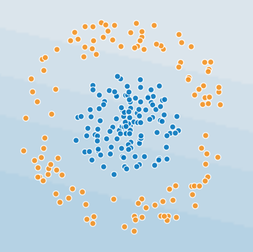
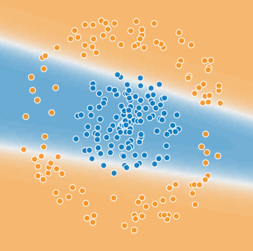
Let’s try a classification problem. We want to train an algorithm to predict which dots are blue and which are orange, based on their position. Imagine we are trying to predict which stocks outperformed the market, using 2 magical factors. Please follow along in the Google TensorFlow playground:

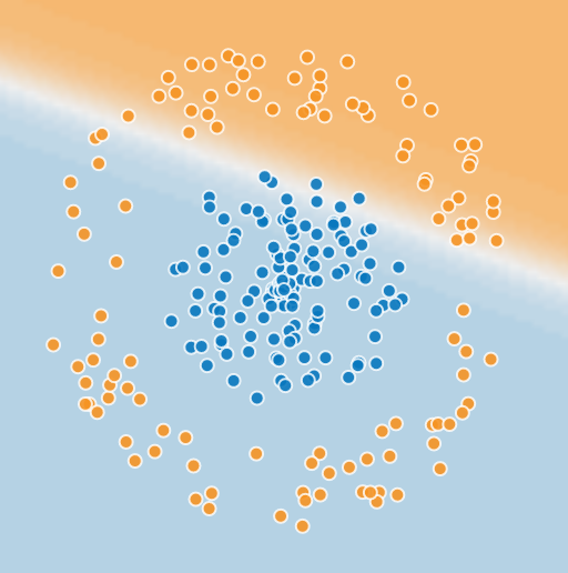
Hit the play button and watch it try to classify the dots using the simplest possible neural network: 1 layer of 1 unit (1×1).

Not very good, but we’ll work on it.

How does this work?

• Our objective is to train a function to predict if an observation is blue or orange based on its position in 2-dimensional space, i.e. using the x and y coordinates as predictors.
• For now, we are using a neural network with a single unit: a 1×1 neural network, 1 layer of 1 cell.
• The cell
  • Takes the x and y coordinates as inputs
  • Applies a linear function of the form ax + by + C to the inputs. This maps any inputs to a number between +∞ and -∞. We’ll call this number O.⁴
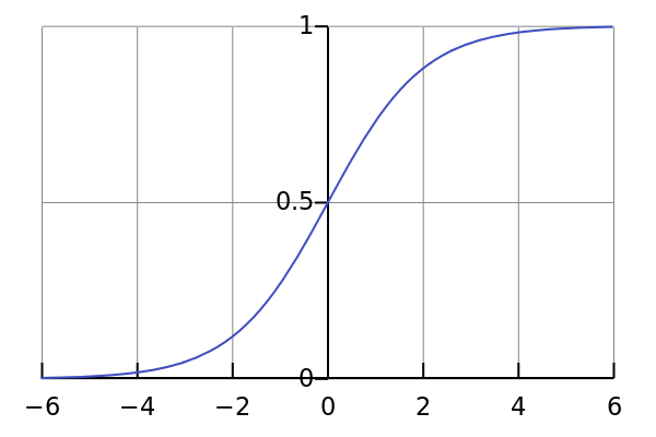
  • Applies a nonlinear function to O called the sigmoid. The sigmoid function maps -∞ to a 100% probability of orange, +∞ is mapped to a 100% probability of blue, and 0 is mapped to 50/50.
  • We estimate the values of a, b, and C that give us the best classifier possible
• To further develop our intuition we can call O “log odds”. If the odds of blue are 3:1, . If the odds of orange are 4:1, .
• We model log odds as a linear function of x and y
• The sigmoid function transforms log odds into probabilities between 0 and 1.
• Therefore the output of our simple network is the probability of blue.

How does the training of this neural network happen, in other words, how do we estimate a, b, and C?

• We initialize a and b to small random numbers, and C to 0 (good places to start for reasons beyond the scope of this introduction).
• We compute a loss function that describes how well this classifier worked. We construct it so if it did well, the error is small, if it did poorly, the error is large.
• We compute the gradient (partial derivative) of the loss function with respect to a, b, and C. In other words we determine if we increase a a little, does the loss improve or worsen, and by how much.⁵
• By descending the gradient we find the values of a, b, and C that reduce the error to a minimum, in other words, we can’t improve in any direction.

OK, what we just did is logistic regression (applied example here). A single-cell neural network with sigmoid activation performs logistic regression and creates a linear decision boundary.⁶
Now add a second cell. Once again, feed x and y to each unit. But now, instead of running the sigmoid on the output of a single cell, we run it on a linear combination of 2 unit outputs. We now have more parameters to estimate…Try it!

We added a second boundary. If x and y are below one boundary, and above the other boundary, classify as blue, else orange.

Add a third cell.

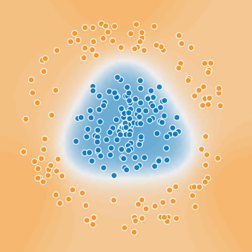
By adding more units, we create a more and more complex boundary.

A single-hidden-layer neural network with sufficient units can approximate an arbitrarily complex decision boundary for classification.⁷ In the case of regression, a neural network can approximate any computable function to any desired level of precision. And, it works for any number of predictors, minimizing error and drawing decision boundaries in n-dimensional space.

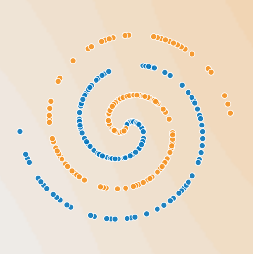
After 3 boundaries, we have a pretty good classifier in this case. But how many do we need in a more difficult example? Look at the image below. How do we determine how many boundaries to add?

The next key concept is…

The bias-variance tradeoff.

As you add variables, interactions, relax linearity assumptions, add higher-order terms, and generally make your model more complex, your model should eventually fit the in-sample data pretty well. And it should generalize to the out-of-sample data pretty well (as a general rule, no better but hopefully not much worse).

But also, as you add more and more complexity to your model, you start to fit the quirks in your training data too well, and your out-of-sample prediction gets worse. You start off being overly constrained by the bias of your a priori model, and then as you add complexity, you become overly sensitive to random variance in the sample data you happen to have encountered.

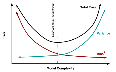
The tradeoff looks like this, via Scott Fortmann-Roe:

Bias is error that comes from underfitting: an overly simplistic, insensitive or otherwise incorrectly specified model. Variance is error that comes from overfitting: from excessive sensitivity to random variation in the sample itself. You have too-sparse data to get precise estimates in your too-numerous parameter estimates. If you happened to pick another random sample your parameter estimates would change.

The data scientist is looking for a good model specification that efficiently uses as few parameters as possible to make the trough in the black line as deep as possible. The good model finds the right bias-variance tradeoff between underfitting and overfitting. But how do we choose this in practice?

Cross-validation, hyperparameters, and test.

The next key concept is cross-validation. Data scientists use careful cross-validation to find the sweet spot in the bias-variance tradeoff, and avoid underfitting or overfitting.

So far we have used one hyperparameter: the number of units in our single layer. We call the number of units in a layer a hyperparameter, to distinguish it from the model parameters we are estimating. Cross-validation is the process by which we tune the values of our hyperparameters to get the best results.

The simplest approach to cross-validation is to take a random 60% of your sample data and make it your training set. Take a random half of what’s left (20%) and make that your cross-validation set. Take the 20% that’s left and make that your test set.

Create a set of hyperparameters to evaluate. In our simple case, vary the number of cells in the hidden layer. For each hyperparameter value, fit the best parameters using the training set, and measure the error in the cross-validation set. Then pick the hyperparameter with the smallest error.

Maybe you have multiple hyperparameters. Perhaps you want to try a neural network of up to 3 10-unit layers. Say for each layer you will try 3, 10, 30, and 100 units.  We have 1 hyperparameter for the number of layers (3 values) and 3 hyperparameters for the number of units in each layer. This yields a grid of something like 4³ (3 layers) + 4² (2 layers) + 4 combinations to test = 64+16+4=84 combinations.

• Loop through all the combinations, training your parameters using the training set only
• Evaluate each model using the cross-validation set only
• Pick the best model

Finally, you may want to evaluate how the model will perform out of sample. To do this, evaluate the final model using the test set. Since you never used the test set to choose a model parameter, this should give you a good estimate of real-world performance.

There are more sophisticated forms of cross-validation: You can split the training + cross-validation into 5 folds. Train 5 times on 4 of the folds, leaving a different fold out each time, measure the error on the left-out fold each time, and then average them. Pick the hyperparameters yielding the smallest average error over all folds. This is called k-fold cross-validation with k=5. It uses your data more efficiently and eliminates the possibility of a lucky or unlucky split between training and cross-validation sets. In the extreme, you can make k=n and leave a single observation out each time… this is called leave-one-out cross-validation. In practice, unless you are starved for training data, k of around 5 is a reasonable balance between maximizing use of the training data, and minimizing computation.

Cross-validating all possible combinations of hyperparameters is a brute-force, compute-intensive process, especially as the number of layers and hyperparameters grows. There are more sophisticated methods like Bayesian optimization, which vary multiple hyperparameters simultaneously, and in theory allow you to find a more finely-tuned best set of hyperparameters with fewer attempts.

The key thing to remember about cross-validation is to make every decision about your model using the cross-validation set. Unlike statistics, where for instance we estimate standard errors based on the assumptions of OLS, any result from training is assumed to not generalize until proved otherwise using cross-validation.

The firewall principle: Never make any decision to modify your model using the test set, and never use the training or cross-validation data sets to evaluate its out-of-sample performance.

The act of using the cross-validation set to choose the hyperparameter values contaminates the cross-validation set for testing purposes. You are most likely to pick a model with pretty good hyperparameters, but you are also more likely to pick a model which also gets luckier in the cross-validation set. For this reason, training accuracy > cross-validation accuracy > test accuracy.⁸ Hence the need for a test set to evaluate the real-world performance of the model. Anytime you use the test set to make a decision about how to use your model, you are tending to turn out-of-sample data into in-sample data.

If you take away one thing from this post, it should be that machine learning allows you to add more noisy predictors, avoid overfitting, and get a fair estimate of out-of-sample performance in the test set. But you need to do it carefully, in accordance with best practices.

That being said, all estimates are overfitted to the data you happen to have. If you train a hot-dog/not-hot-dog classifier, and in your training data, only hot dogs have ketchup, then your classifier may learn that ketchup means hot dog. The higher the risk that your training data may not be totally representative, that the future may not be like the past, the more you should err on the side of underfitting.

Regularization, ‘worse is better’, and other stupid tricks.

Data scientists improve the bias-variance tradeoff by using cost functions that are able to find good predictive signals while filtering noise.

This part always blows my mind a little. As we’ve seen, a good machine learning model is a model with a good bias-variance tradeoff: a low minimum in the cost function, resulting in a small error in cross-validation. If you can find methods that make the model inherently resistant to chasing noise in the data, without disturbing the essence of prediction, you get a good bias-variance tradeoff.

A simple method is regularization. When an estimated parameter gets large, that may be because it captures a highly significant relationship. Another possibility is it got lucky with this dataset and just happens to be strongly correlated with its random variation.

The regularization ‘stupid trick’ is to add a penalty for each parameter to the cost function, that typically scales linearly (L1 regularization) or quadratically (L2 regularization) with the regularized parameter. This shrinks large parameters, whenever increasing the parameter doesn’t correspondingly improve the cost function.

Lo and behold, we almost always find that by making the model perform worse in-sample, it performs better out-of-sample. This is particularly true when you have noisy, multicollinear data. Regularization reduces the impact of the noise and builds redundancy over the correlated variables.

The lasso regression is a popular application of regularization (applied example). You use a linear regularization and start with an unlimited ‘budget’ on the regularization cost, i.e. the sum of the linear parameters multiplied by the regularization hyperparameter. Then you gradually shrink the budget. The regression will shrink the parameters that have high costs but don’t improve the prediction much. Gradually it shrinks some parameters to zero, throwing out predictors and performing implicit variable selection. You keep shrinking the budget until you find the right bias-variance tradeoff.

There are some amazingly creative worse-is-better tricks in machine learning. Random forest is a ‘worse is better’ variation on decision trees.

A tree is an algorithm where you take a set of predictors, and you look for the best rule of the form ‘When return on equity is greater than x, book value is less than y, PE is less than z, and momentum is higher than α… classify as X‘. When you use a random forest, instead of finding the best decision tree possible with all the predictors in you data set, you throw out a random half of your predictors; find the best tree that uses only those predictors; repeat this process 10,000 times with a different random selection of predictors; and have the 10,000 simplified trees (the ‘random forest’) vote on the outcome. That turns out to be a better tree than the one using all the data. Crazy.

One reason it works is that it doesn’t become overly reliant on any one set of indicators, so it generalizes better out-of-sample.

Similarly with neural networks, you can use L1 or L2 regularization on all your parameters, but even more creatively, throw out half your units each training iteration, and call it dropout. Dropout forces the other activations to pick up the slack and builds redundant reasoning. Then do cross-validation with the entire network. It’s like Bill Bradley training to dribble with glasses that blocked his view so he couldn’t look down at the ball (and lead weights in his shoes).

Finally, you can use ensemble methods. First classify your data with a neural network, then with a random forest. Then use logistic regression to classify using the results of the previous two methods.
It’s not always obvious at first glance why some of these tricks work, but in general, they make it harder for the algorithm to chase quirks in the data, and improve out-of-sample performance. Finding clever ways to make your algorithm work a little harder for worse results in training can make it work better in the real world. Maybe you can see why one might call it street-fighting statistics.

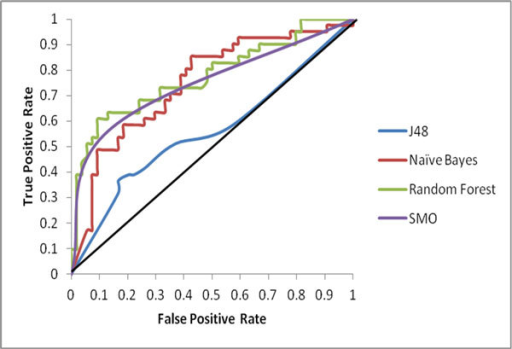
The ROC curve helps us trade off false positives against false negatives, and find the most efficient classifier for a given problem.

Suppose I told you that I have a classifier that accurately classifies CAT scans as cancer/not cancer in 99% of cases. Is that good or bad? Suppose only 1% of scans are cancer. Then it’s not very good: we could get the same accuracy by classifying all the scans as healthy. We need a measure of classifier quality that takes into account the base rate (1% incidence of cancer), the classifier’s rate of false positives, and the rate of false negatives.

The ROC (Receiver Operating Characteristic) curve came from analyzing radar data in WW2. If your radar receiver detected a radar return, it could classify it as an incoming aircraft, or as noise. If you made the receiver extremely sensitive, you would detect all the incoming aircraft (true positives), but you might also detect a lot of birds and random static (false positives). As you decrease the sensitivity, you reduce the false positives, but you also increase the false negatives, simultaneously increasing the chance of missing a real aircraft.

Here’s an example from published research:

If 50% of the incoming data are labeled true and 50% false, and if you have a classifier with no real information rate, for instance, you classify observations randomly at the 50% base rate, then the ROC curve will be a 45° line.

If you have a better classifier, it will be curvy and convex with respect to the best case of 100% true positives and 100% true negatives (top left). If you have a really great classifier, the ROC curve will be a very sharp right angle. If it’s better at avoiding false positives or negatives, it may skew in one direction or the other.⁹

The area under the curve (AUC) is a measure of overall classifier quality. A perfect classifier has a AUC close to 1, a poor classifier close to 0.5 in this example.

By selecting a threshold above which you classify as true, you can vary the sensitivity of your classifier. If the cost of a false negative is very high, you might set a low threshold and have high sensitivity (% of positives correctly classified: true positives). If the cost of a false positive is very high, you set a high threshold and low sensitivity and high specificity (% of negatives correctly classified: true negatives). You have to balance the possibility of being bombed against the possibility of launching all your expensive missiles at seagulls.

If the cost of a false positive always equals the cost of a false negative, you set a threshold to simply minimize the total number of errors, whether false positives or negatives. If the cost of a false positive is not the same as the cost of a false negative, you can minimize the total cost by increasing the threshold until the cost of false positives avoided equals the cost of false negatives added¹⁰.

Deep learning

Modern GPUs and efficient algorithms allow us to combine these building blocks into complex stacks. Deep learning networks of more than 1000 layers are trained end-to-end to solve increasingly complex problems with human-like intelligence.

Mind-blowing examples, such as facial recognition and natural language processing like Siri, seem indistinguishable from magic, but can be decomposed into a series of tractable steps.

Try this image labeling demo. It’s simple enough to run in your browser. The architecture is complex: a series of convolutional layers that essentially scan for specific features, interspersed with rectified linear layers and max pooling layers that select the highest scoring ‘convolution’ or scan offset. The layers toward the left look for low-level features, and as you move toward the right, you look for increasingly complex combinations of higher level features.

The hallmark of deep learning is that you train a very deep neural network with potentially hundreds of layers, each architected to solve a stage of the problem, and you train the entire network end-to-end.
Before neural networks, a state-of-the-art (SOTA) machine translation effort might consist a series of stages:

• Parse words and preprocess them (remove punctuation, common misspellings, maybe combine common n-grams or word combinations
• ‘Stem’ the words and classify by parts of speech, in other words ‘parsing’ -> ‘to parse’, verb, gerund
• Find a distribution of possible corresponding individual words and n-grams in the target language
• Try to diagram the sentence, build a graph of how the parts of speech relate to each other
• Given a distribution of possible sentences, and a language model that allows one to estimate the probability of different sentence structures and word co-occurrences, compute a probability distribution and identify the most likely full sentence in the target language.

Each task might have a couple of Ph.D.s and the whole team might be dozens of engineers working for a year.

With a neural network, you start with a parallel corpus of several hundred books worth of e.g. English and French, you set up a network of, for instance, 16 layers. You need a cost function that evaluates the quality of the translation. You repeatedly translate chunks, evaluate the gradient of the cost function across the entire network, and adjust your parameters. For a large network, this might take weeks, even spread out over hundreds of GPUs in a cluster of computers.

End-to-end training of the entire network against the task-specific objective is the key to deep learning:

• Each layer optimizes activations directly against performance on the ultimate task.
• The optimization takes into account what other layers upstream and downstream are doing, and how they jointly impact the cost function and gradient.
• Complex interactions between layers emerge, optimized for the task at hand.
• Modern GPUs supporting massively parallel computation, and relatively efficient algorithms¹¹ allow computation of gradients to optimize large deep networks.

When you train a deep learning network end-to-end, the training process starts to feel like intelligent learning. Every new batch of data is analyzed for how to improve the whole process, and complex new features and interactions between layers start to emerge.

The end result is that the network seems to come alive, layers find high-level features to look for in the noisy data, and the system teaches itself to translate almost as well as human translators, and better than systems manually fine-tuned by teams of engineers.

Concluding remarks

These are the key concepts we’ve discussed:

• The cost function and gradient descent
• The bias-variance tradeoff
• Cross-validation and hyperparameter selection
• Regularization
• The ROC curve

If you understand them, you are off to a good start in your machine learning adventure.
The following heuristic should apply: If your data match the assumptions of OLS, machine learning should give you the same results as when you use linear regression. If your data don’t match the assumptions of OLS, if you have a lot of noisy data with nonlinear relationships and complex interactions, you’ll probably get some improvement with machine learning tools. Sometimes a little, sometimes a lot.

So, if your goal is the best possible predictions, and you have lots of noisy data that violate assumptions of OLS, it is worthwhile to understand the machine learning approach. In comparison with traditional statistical methods, one can argue that machine learning is the least Bayesian approach, since it can dispense with not only any prior distribution, but also any notion of an ideal variable or a priori functional form of the solution. It simply asks how to minimize some error or cost function defined in reference to a task.

Machine learning targets prediction; if it has an Achilles heel, it is attribution.¹²

When you model a variable with multiple layers of complex non-linear interactions, it becomes impossible to explain why the model made the choice or estimate it did. For many applications, it doesn’t matter. You don’t really care why your phone’s predictive text made the prediction it did (as long as it worked). But when parole boards apply machine learning to score applicants for early release, data quirks can easily lead to arbitrary or inappropriately biased decisions.

When we do economics, we combine theoretical models and empirical evidence. If all you do is derive models from first principles, they usually don’t match the real world very well. If all you do is study past relationships, you don’t have a framework to understand what happens when anything changes beyond past relationships. So typically you write down a model that uses a theory to encapsulate the dynamics of the system, and then you estimate parameters using econometrics. This enables you to reason about what will happen if you change the underlying system through policy. If you don’t have a theoretical framework, you don’t know why things happen. And you can’t predict anything that doesn’t closely resemble the past.

If you apply machine learning to credit decisions, it might decide that people of certain ethnicities or living in certain geographical locations, or who have Facebook friends with bad credit, are poor credit risks. It might tend to exacerbate arbitrary existing patterns.

If your data represent existing social biases, the algorithm will tend to learn those biases. If your data is not representative, the algorithm will make poor predictions.

Investing needs heart as well as mind; theory as well as pattern recognition; wisdom, fortitude and nerve as well as analytical power. Long-term asset allocation isn’t necessarily a great candidate for machine learning. There’s a lack of sufficient data, a need for attribution, and a future which may not be like the past.

But for much of what investors do, AI helpers will be the rule rather than the exception. It’s already happening in applications from stock screening for further analysis based on the stocks a manager typically looks at, to technical analysis and developing algorithms for short-term trading against other machines.

In the not-too-distant future, AI will be assumed as a basic part of the investor toolkit, and managing without it will be unthinkable. We will see more amazing applications…possibly new theoretical breakthroughs and investing paradigms…and probably a few disasters along the way as well.

Some fun examples, and a roadmap for study

The next steps are to pick a problem, write some code, maybe take an online course, dive into more complex algorithms like RNNs, CNNs, reinforcement learning.

Simple finance examples with code to get you started:

• Equity premium prediction with R. To run it, get git, clone the GitHub repo and run with R-Studio
• Equity premium prediction with Keras/TensorFlow. To run it, get the Anaconda distribution, clone the GitHub repo, and run with Jupyter. (R is the training wheels and Keras/TensorFlow is the road bike.)

Amazing examples:

• Quick, Draw – See if Google can recognize your doodle. By looking at enough doodles, Google can analyze the data and teach its own algorithm to doodle.
• Deep Art style transfer.
• Uncanny arithmetic on representations of words with Word2Vec and faces with generative adversarial networks.
• What your self-driving car sees.
• More examples

Primers

• Andreessen Horowitz AI playbook
• AI Revealed, via Yann Le Cun and Facebook Code
• Jon Krohn
• Alfred Spector
• Machine Learning Mastery – Jason Brownlee (Many excellent tutorials on specific algos)
• More tutorials and primers

Books and courses

• Hands-On Machine Learning with Scikit-Learn and TensorFlow, Aurélien Géron
• Deep Learning, Ian Goodfellow and Yoshua Bengio and Aaron Courville
• Stanford CS 20SI: TensorFlow for Deep Learning Research
• Stanford CS229 Machine Learning (Andrew Ng intro course)
• Stanford CS221: Artificial Intelligence: Principles and Techniques (Percy Liang intro course)
• Stanford CS231n: Convolutional Neural Networks for Visual Recognition (Image processing)
• Stanford CS224n: Natural Language Processing with Deep Learning
• More courses and books.

References

¹ Noteworthy and not atypical implementation details: A surprisingly complex trial-and-error process; a complex solution that looks deceptively simple.
² These three unsupervised learning tasks are somewhat closely related. If you can tell how things are similar in the important features, you can tell which ones are different, and throw away the noise.
³ One could view reinforcement as a type of iterated supervised learning where you sample more complex inputs and outputs, or where you attempt to learn a higher-level objective like playing a game or driving a car through trial and error, using the same techniques as classification and regression. But it’s considered sufficiently different and important that many people put it in its own category.
⁴ For simplicity, we’re not using a ‘standard’ notation, which exist using several conventions with scary Greek letters.
⁵ We can’t apply gradient descent to accuracy directly, because it’s discrete. If you change your model an infinitesimal amount, it won’t change any individual prediction directly. The cost function is a smooth, differentiable function that we can apply gradient descent to, that is a good proxy for what we are trying to minimize, in this case inaccurate classifications.
⁶ Logistic regression is a generative method, in that for any x and y, it generates a numeric probability. A discriminant method just comes up with a boundary. Using logistic regression to come up with a linear decision boundary is equivalent to linear discriminant analysis.
A note on activation functions. The Google playground gives a choice of activation functions including sigmoid, tanh, and ReLu. The sigmoid function has an intuitive mathematical foundation: if in fact the log odds are some piecewise linear function of the coordinates, our neural network will converge on correct probabilities. But any of the nonlinearities can approximate any arbitrarily complex boundary with sufficient units. If you try them, you might find that the other nonlinearities converge faster: tanh (squashes -∞ to +∞ down to -1 to +1) and ReLu (rectified linear unit, makes everything above 0 linear and everything else 0. Which one works better might depend on the problem, one might just be faster because it’s less complex to differentiate and optimize.
⁷ In practice, when a problem is amenable to being solved in steps, a multi-layer deep network is more common than single-layer. Layers end up performing different tasks, e.g. edge detection, detection of complex objects with many edges, object classification.
⁸ For the same reason, if there is a cross-validation that is not significantly worse than the best, but with more bias and less variance, you are usually better off selecting its hyperparameters.
⁹ If one method is good at avoiding false positives and another at false positives, what does that tell you? Time to use an ensemble method combining both!
¹⁰ If you reverse the y-axis of the ROC curve you can set a threshold where the slope equals the relative cost. The f score is an alternative approach.
¹¹ Backpropagation is the name of the algorithm that lets you efficiently compute all the gradients in a single pass, where earlier gradients depend on later gradients (or vice-versa depending on how you look at it.
¹² People are working on this. One can, of course, make small changes in the inputs and see how they affect outputs. But the point of machine learning is to find complex nonlinear relationships and interrelationships. So the whole model may act in ways that are hard to explain or to justify.