Buy cheap.
This is a motto many live by, not only in their daily lives but also in their investment philosophy. Historically, “buying cheap” stocks was a good idea (i.e., the so-called “value” premium).
But how might valuation matter when it comes to country allocations? In other words, given valuations, how much money should I allocate to U.S. equity and how much should I allocate to International equity?
There is no right or wrong answer here. Some, such as Warren Buffet, recommends ~100% U.S. exposure (as of 2017). However, as we have discussed here, the high U.S. equity returns may be anomalous.
So given current valuation information, and knowing that diversification is the so-called “free lunch” of investing, how can one approach the U.S./International allocation decision?
Two simple solutions are generally offered:
- Allocate according to overall market-cap of the respective markets. This is currently around 52% U.S. and 48% Developed International.
- Split the assets evenly — 50% U.S. and 50% International.
Both are decent approaches to this decision.
But what about allocating capital based on “cheapness”? In other words, value-investing across equity exposures.
There are numerous papers/articles written on this topic. A few of them are by AQR (and affiliates), Meb Faber, Research Affiliates, and Newfound Research.(1) While the referenced studies use different measures of value, in general, they have found that in the past value investing has worked across country allocations–meaning “cheaper” countries outperformed “expensive” countries (on average).
Assuming one buys the argument of valuation-based timing, a natural question is to ask which valuation metric works the best?
A new paper, titled “And the Winner Is… A Comparison of Valuation Measures for Country Asset Allocation,” by Adam Zaremba and Jan Jakub Szczygielski asks this exact question. The paper can be found here.
Below we dig into the paper.
The Results
The paper begins by reviewing the different measures used in the literature to split firms into value and growth. The authors split firms based on a “yield” measure, using seven variables as the numerator and two variables as the denominator:
Below are the seven numerator variables:
- Earnings
- Book Value
- Cash Flow
- EBITDA
- Gross Profits
- Sales
- Dividend
Below are the two denominators variables:
- Market Capitalization
- Total Enterprise Value
So in total, the authors examine 14 measures (and the EW-combinations) by taking each of the seven numerator measures and dividing these by either Market Capitalization or Total Enterprise Value. The country values for the measures, such as EBIDTA/TEV, is computed in the paper using Bloomberg Data for the underlying stocks (at the firm level) and then weighting each firm by its respective weight in the index.
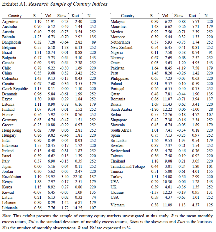
The paper first examines the returns to 73 countries, including both developed and emerging countries.(2)The time period is a 21-year stretch, from May 1996 – April 2017. The paper first examines the country returns via a Fama-MacBeth regression and finds that, not surprisingly, value and momentum are predictive of future returns. The paper then splits firms into thirds based on each measure, and examines the returns to the terciles, from cheap to expensive.
The results are shown in Exhibit 2 and below:

The results are hypothetical results and are NOT an indicator of future results and do NOT represent returns that any investor actually attained. Indexes are unmanaged, do not reflect management or trading fees, and one cannot invest directly in an index. Additional information regarding the construction of these results is available upon request.
The table is split (from left to right) based on either using (1) Market Capitalization or (2) Total Enterprise Value (TEV) as the denominator. When examining Panel A, one finds that Value (Top) outperforms Growth (Bottom), or cheap outperforms expensive.(3)
In order to determine how tradable this strategy would be (over this time period), the paper examines the same strategy while using 42 iShares ETFs listed below:
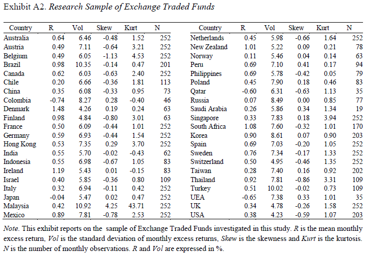
The results are hypothetical results and are NOT an indicator of future results and do NOT represent returns that any investor actually attained. Indexes are unmanaged, do not reflect management or trading fees, and one cannot invest directly in an index. Additional information regarding the construction of these results is available upon request.
As is shown above, some of the ETFs are not in the sample for the entire time period (Saudi Arabia is only in the sample for 19 months). The authors assume cost estimates of (1) 0.07% for trading commissions and (2) half of the bid-ask spread.
The results after accounting for trading costs (and on the smaller 42-country universe) are shown in Exhibit 3 and below:
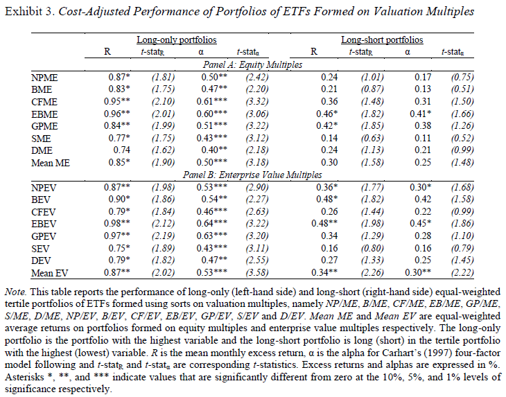
The results are hypothetical results and are NOT an indicator of future results and do NOT represent returns that any investor actually attained. Indexes are unmanaged, do not reflect management or trading fees, and one cannot invest directly in an index. Additional information regarding the construction of these results is available upon request.
The table highlights that the long-only portfolios had (1) positive returns and (2) positive alphas. This makes sense as the portfolios (1) had allocations to equity and (2) can be long international stocks whose returns may not get picked up by the U.S. 4-factor regression. So both of those observations are somewhat expected.
Examining the long-short portfolios, one notices that the mean EW portfolios work appear to work better using TEV as opposed to Market Capitalization as the denominator. Additionally, if one had to select a specific measure, the EBITDA/TEV measure worked the best over that sample period. This is similar to what we found in U.S. stocks from 1971-2010 (although EBITDA/TEV did not work well recently).
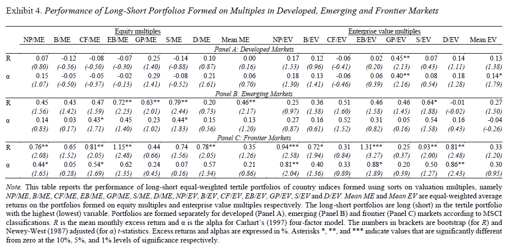
However, the paper wanted to dig deeper and see how the performance varied across (1) developed, (2) emerging, and (3) frontier markets.
The results are shown in Exhibit 4 of the paper and below:
The results are hypothetical results and are NOT an indicator of future results and do NOT represent returns that any investor actually attained. Indexes are unmanaged, do not reflect management or trading fees, and one cannot invest directly in an index. Additional information regarding the construction of these results is available upon request.
As is shown above, the long/short portfolios generally worked the best in frontier and emerging markets. However, the mean EW portfolios (all the measures) using TEV in the denominator are not significant for both frontier and emerging markets, while only significant using Market Cap in the denominator for emerging markets. Examining developed markets, there is very little significance amongst the L/S portfolios, save the GP/TEV variable. Now one needs to caveat the results with (1) small sample size and (2) relatively small time window–but that being said, it appears valuation-timing works the best in emerging and frontier markets.
Next, the paper splits the time period approximately in half and examines the returns to the long/short portfolios between (1) June 1995 – May 2006 and (2) June 2006 – April 2017.
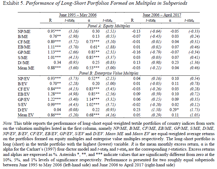
The results are hypothetical results and are NOT an indicator of future results and do NOT represent returns that any investor actually attained. Indexes are unmanaged, do not reflect management or trading fees, and one cannot invest directly in an index. Additional information regarding the construction of these results is available upon request.
While this sample now includes all of the markets, one thing is clear–the majority (or all!) of the returns to the long/short country portfolios on valuations occurred within the first time-period. The second time-period has almost no significant returns or alpha. To emphasize this point, the authors create a graph plotting the cumulative returns to the long/short portfolios.
This is shown in Exhibit 6 of the paper and below:
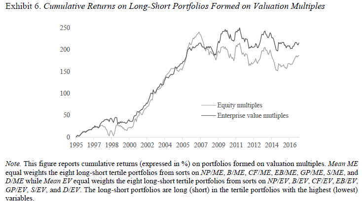
The results are hypothetical results and are NOT an indicator of future results and do NOT represent returns that any investor actually attained. Indexes are unmanaged, do not reflect management or trading fees, and one cannot invest directly in an index. Additional information regarding the construction of these results is available upon request.
Overall, the picture fits a narrative that has been true for some time now, which is that country valuation based-timing models have not worked too well (since 2006).
Conclusions
As is shown in the cumulative returns graphs above, country valuation based-timing strategies have not worked for some time now! Any advisor(4) who advocates a decent international exposure knows that the U.S., while more expensive than other markets, has been on a great 9-year run now, trouncing developed and emerging equities.(5) So is Warren Buffet right–should we put 100% in the U.S.?
I would still advocate against such an approach and prefer a ~50/50 allocation, but as with anything investing, nothing works all the time. For those really interested in this topic, I recommend you read some more of the Research Affiliates articles, such as here, here, and here. In addition, they have a great tool that allows investors to investigate projected future returns for multiple asset classes (with assumptions and different models).(6)
Let us know what you think …
And the Winner is … A Comparison of Valuation Measures for Country Asset Allocation
- Adam Zaremba and Jan Jakub Szczygielski
- A version of the paper can be found here.
- Want a summary of academic papers with alpha? Check out our Academic Research Recap Category.
Abstract:
The authors evaluate and compare the usefulness of various valuation ratios for country selection. To this end, the performance of 73 national equity indices is investigated for the period 1996 to 2017. The EBITDA-to-EV multiple is the best predictor of performance and outperforms other metrics. An equalweighted portfolio that is long (short) in the tertile of countries with the highest (lowest) EBITDA-to-EV ratio produces a mean monthly return of 0.69% and a Sharpe ratio of 0.81. These are more than double the Sharpe ratios obtained from using traditional metrics such as the book-to-market ratio or dividend yield. Two major drawbacks of inter-country value strategies are identified: 1) payoffs are derived predominantly from emerging and frontier markets and 2) profitability has significantly declined in the last decade.
References[+]
| ↑1 | To be fair, only including those four links is only a small amount of research that has been examined on the topic. Nevertheless, I include them as references worth reading. |
|---|---|
| ↑2 |
The list of the countries can be found here:
The results are hypothetical results and are NOT an indicator of future results and do NOT represent returns that any investor actually attained. Indexes are unmanaged, do not reflect management or trading fees, and one cannot invest directly in an index. Additional information regarding the construction of these results is available upon request. |
| ↑3 | Panel B then examines the 4-factor Alphas, and one can argue that there is more “alpha” for the TEV portfolios. |
| ↑4 | Including us!! |
| ↑5 | 2017 was a change, but who knows how long that will last. |
| ↑6 | Note: predicting asset class returns is hard. |
About the Author: Jack Vogel, PhD
—
Important Disclosures
For informational and educational purposes only and should not be construed as specific investment, accounting, legal, or tax advice. Certain information is deemed to be reliable, but its accuracy and completeness cannot be guaranteed. Third party information may become outdated or otherwise superseded without notice. Neither the Securities and Exchange Commission (SEC) nor any other federal or state agency has approved, determined the accuracy, or confirmed the adequacy of this article.
The views and opinions expressed herein are those of the author and do not necessarily reflect the views of Alpha Architect, its affiliates or its employees. Our full disclosures are available here. Definitions of common statistics used in our analysis are available here (towards the bottom).
Join thousands of other readers and subscribe to our blog.