Assume you made a decision to invest in an active strategy based on, say, a backtest of the underlying process (to be clear, active means NOT passive market-cap weight in my context). Over the next few years, you sit in the strategy watching it underperform the passive benchmark. You are a disciplined investor, so you don’t want to dump something based on recent performance, but you also don’t want to ride a losing strategy until you end up in bankruptcy court.
How does one take this recent information and rationally update their assessment of the underlying process?
In principle, that insight should be based on the magnitude of underperformance, the length of underperformance, and the initial conviction to the decision to invest in the asset (your “prior”). This is in line with Bayesian thinking and also seems quite intuitive. However, often in practical portfolio management, the data based on 3- or 5-year track records is evaluated (AA summary) without taking the initial investment conviction into account. Actually, some research suggests that even three years of underperformance may be too long to be tolerated for some individuals. Obviously, the investment conviction is either 1) very weak or 2) non-existent if several years of underperformance makes one change their mind. I argue that the conventional practice of chasing the past 3 to 5 years of past returns is suboptimal. But why?
Cam Harvey from Research Affiliates has expressed this much better than I ever could, so I’ll just simply quote him on the matter:
Imagine that a musicologist correctly distinguished 10 out of 10 pages of music as being written either by Mozart or by Haydn. Also imagine that a kindergartener calls 10 coin flips correctly. Would you be as convinced of the child’s skills as you would be of the musicologist’s? I would hope the answer is “no” because you have a prior on the skills brought to the task, as opposed to being simple luck. Priors aren’t perfect (who knows, maybe the five-year-old is a budding fortune teller…), but they are very helpful.
Interpreting the message for an investment track record analysis is equivalent to ignoring the prior (the reason why we invested in the first place) and making portfolio management decisions solely based on realized investment under(over)-performance. In what follows we’ll outline how an investor can use Bayesian probability theory to make (arguably) more informed decisions.
Here are the key points we’ll address:
- What to do with underperforming investments? This is a question that often pops up. As you’ll see, it is actually surprisingly simple to apply Bayesian inference to get an informed answer to that question
- Bayesian priors are subjective but it does not mean that we couldn’t or shouldn’t use analytical methods in a transparent manner to express them
- Short track records are often significant only in isolation without considering the initial conviction to the investment decision
Bayesian Probably Theory?
What is Bayesian probably theory? Well, there are two main schools of thought in statistics: Bayesian and frequentist. The chief difference between the two is the use of a prior. While a frequentist calculates the probability solely based on available data, a Bayesian takes the subjective prior beliefs into account as well. Hence, a Bayesian openly admits that probability is a subjective quantity. Traditionally, fund track records are analyzed in isolation, without considering the prior, that is, as frequentists like to do. That wouldn’t be a big issue if there were plenty of multi-decade live track record data available. But this isn’t the case. Track records are typically less than 10 years. But when a track record is short, in most practical cases, the choice of a prior, matters a lot. Now, I cannot resist the temptation to spoil the surprise, track record analysis with Bayesian inference is actually quite simple. But before digging into the good stuff, it probably makes sense to see how track records are traditionally evaluated via the frequentist methodology.
The Frequentist Approach for Evaluating Track Records
To make this more applied, I have chosen the QV index (U.S. Quantitative Value, net of 2% assumed frictional costs) as a case study.
(1)QV reflects a highly active systematic value investing strategy that most readers of this forum are probably familiar with (see here for an overview of the process). The analysis that follows doesn’t aim to reveal whether QV index is a “good” or “bad” investment, but rather, serves as a great introduction to frequentist versus Bayesian inference.
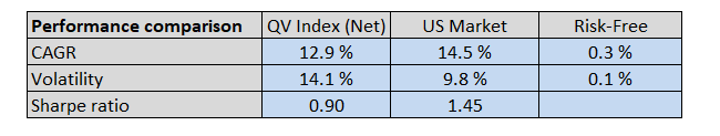
Now, let’s start by comparing the QV Index (Net) to the passive market-cap-weighted US stock market index (data from AQR) since 1/1/2013.
- QV Index = U.S. Quantitative Value Index, net of 2% in assumed frictional fees.
- US Market = Market-cap weighted US Stock market. Gross of fees.
- Risk-Free = U.S. Treasury Bills. Gross of fees.
- Total returns, including dividends and distributions
Looking at the results below, we can see that QV index has underperformed US stock market since 12-2012 when the Quantitative Value book was published. That is five years of live underperformance. The conclusion remains the same whether we measured the performance as compounded annual growth rate (12.9% vs. 14.5%) or risk corrected by Sharpe ratio (0.90 vs. 1.45). In short, from January 1, 2013, to December 31, 2017, the strategy had underperformed a passive index.
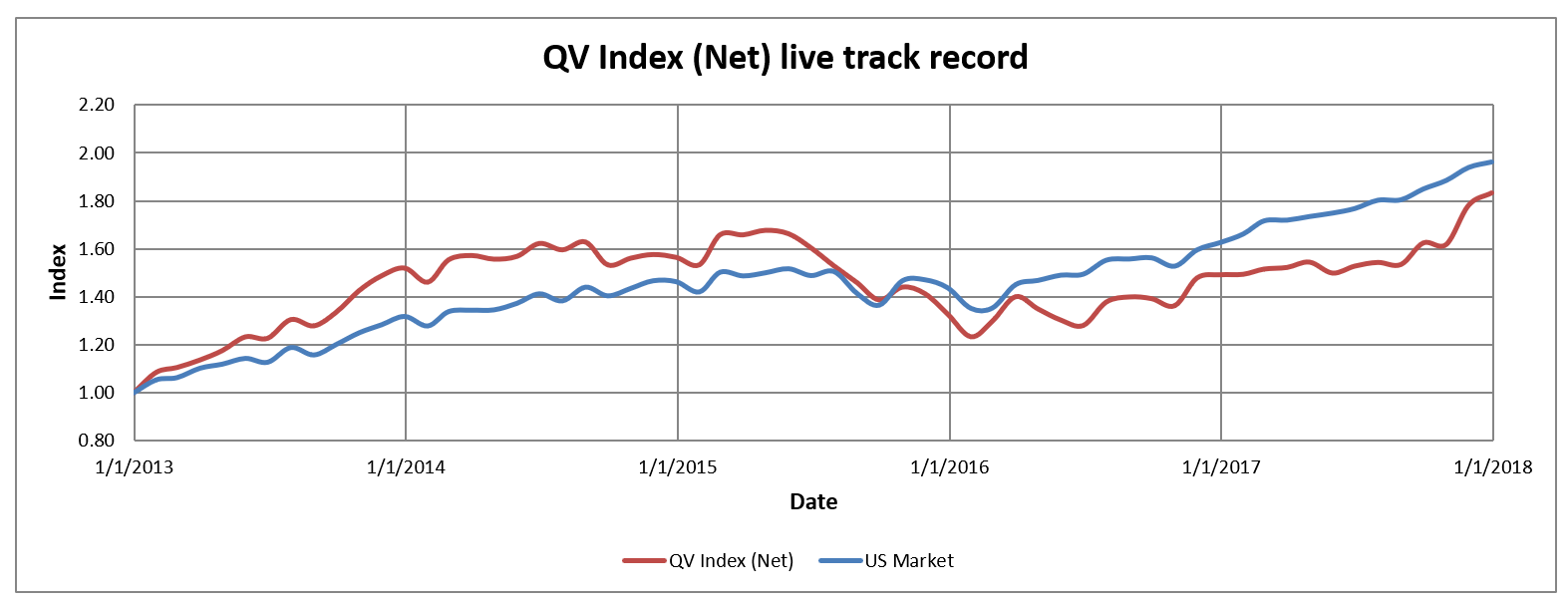
Here is the invested growth chart comparing the QV Net Index against the US stock market index:
Next, let’s calculate a measure of annualized alpha (relative performance compared to a benchmark) and tracking error (active risk) for the QV Index (Net) since it went live. In order to create a simple alpha estimate, I simply take the difference in the compound annualized growth rates between the QV Index (Net) and the US Market. This approach to calculating “alpha” isn’t the typical regression approach, but it is good enough for our purposes. We also calculate the standard error of the mean (SEM), which is simply the tracking error scaled by the square root of time (number of years in the track record). Annualized alpha and SEM can be then used to estimate the frequentist probability that the strategy of QV is better than it’s benchmark. I do that by applying the cumulative density function of the Gaussian distribution defined by alpha and SEM.
Say what?
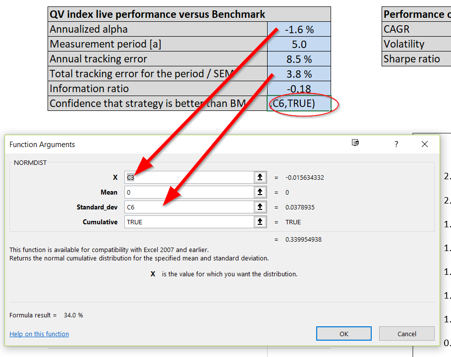
I simply mean, this can be done by using the common, “NORMDIST(alpha,0,SEM,1)” function in excel. This function will spit out the probability of seeing the observed alpha estimate (i.e. “alpha”), under the null hypothesis that the true alpha mean is zero and the alpha estimate’s volatility (i.e., “SEM”). The final “1” in the function simply tells excel that we want to look at the cumulative distribution.
The image below should help readers understand how the function is deployed:
The information that comes out from this analysis is below:
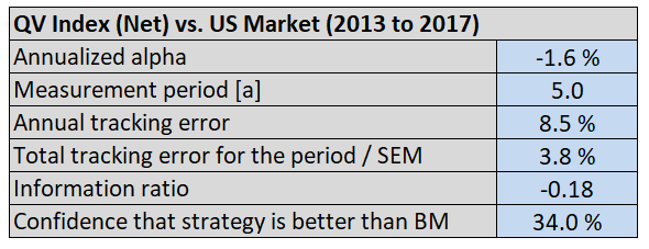
Based on this track record analysis from 2013 to 2017, and after plugging our estimates into the Normdist function, we identify that there is approximately a 66% (100% – 34.0%) probability that the actual alpha for QV index is negative.
Sell, sell, sell?
The probability generated can be seen as a number quantifying the role of luck in the realized track record. In principle, if we are more than 50% confident that the actual alpha of our investment is negative, we should sell the asset and replace it with something else (neglecting trading frictions and taxes embedded on the decision). Alas, this analysis approach is what many investors seem to do when they see 3-5 years of underperformance.
Of course, that would be a rational decision only if the track record was the only source of information for the decision-making. Essentially, this can only be the case if the decision-maker has no prior, meaning that those investors (assuming they are rational) must have initially decided to pick the investments randomly. Now to think of it, maybe there are some investors who do this: use a random generator to pick funds. In this scenario, the frequentist analysis above is adequate and these investors should rationally stop following the QV Index!
Everyone else, who conducts research and analysis before undertaking an investment decision and establish a prior, should consider what Mr. Bayes has to say about the QV Index (Net) track record from 2013 to 2017.
Bayesian Story of the Lost Prior
These days everyone talks about rationally updating their beliefs when new information becomes available. In other words, they consider themselves to be a “Bayesian updater”.
(2)However, it is rare to see anyone apply this approach in a transparent way. Maybe that is because of that disgusting need for a so-called “prior,” which drives people nuts. Priors, you see, are subjective. Even the word subjective can cause chills for a data-oriented evidence-based person. Luckily, I have good news for such an individual, subjective views can also be based on data!(3)
And the bad news? Complete objectivity of the data science is a fallacy!
Why? Because data analysts make all kinds of subjective decisions along the way when they are interpreting the data. However, let’s not go down that rabbit hole of esoteric debates in statistics, but rather, let’s concentrate on understanding how to define the subjective prior as objectively, or at least reasonably, as possible.
We’ll need a pinch of imagination to come up with a subjective investment prior in order to complete our little case study. For the sake of argument, say, on the December 2012 publication date of the book, “Quantitative Value,” which outlines the philosophy behind the QV Index (Net), we instantly went out and started following the QV Index (Net) strategy.
But why did we make that investment decision? If the decision was based on a random generator, there is no need to continue with the Bayesian analysis. However, for the rest of us, our decision to use the QV Index must be because we had conviction in that decision before making it. In other words, we established a prior. Maybe our thinking went along these lines: we used to believe in efficient markets (prior), but then we stumbled on this new QV Index approach, which has a compelling 39-year backtest (evidence), which made us change our mind.
Let me try to quantify that “prior” paragraph (sorry, a bad stat joke!).
The prior was that the expected alpha of any investment strategy should be 0% (efficient markets hypothesis or EMH). But, we couldn’t be sure, because some of the more recent academic studies had suggested that some market opportunities may still remain due to limits to arbitrage and/or behavioral biases. Say the confidence of our market efficiency prior can be quantified to be 2% in terms of standard deviation. That is, we were 95% certain that the annual alpha (true alpha, without noise) of any investment strategy should be between -4% and 4%. That’s it, a form of the efficient market prior, quantified. Now, you may disagree with the choice of this prior and that is perfectly okay because, by definition, priors are subjective. However, in order to complete the case study, we need to pick and quantify a prior.(4)
Now let’s look at the evidence presented via the QV Index backtest. Imagine we see this evidence over the January 1, 1974 to December 31, 2012 period. The backtested annual alpha of the strategy was 6.1% after fees with 10.1% tracking error.
Here is the invested growth chart:
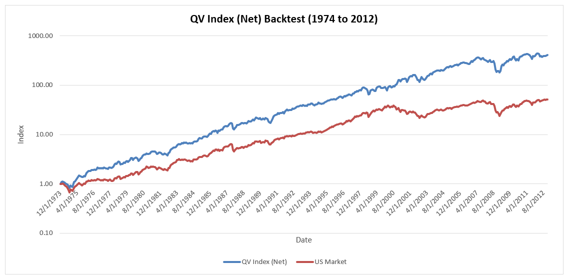
And here is the table of summary statistics:
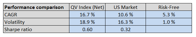
Well, of course, when Wes showed us the backtest we didn’t quite believe him!
We had our prior belief regarding market efficiency (defined above). In addition, we did our homework and read the research on backtests. The research says that one should apply some haircut when evaluating backtested results to compensate for the usual suspects like trading frictions, data mining and increasing market efficiency. Wes had actually done some haircutting for the QV Index and had already taken 2%/year off the top due to expected frictions and management fees. Still, we wanted to be conservative and based on our skepticism of backtests we decided to go with the typical 50% alpha haircut, after which, 3.0% annual backtest alpha remains.
Let’s stop for a moment to summarize the situation:
- We had backtested data from AA and benchmark data from AQR.
- The efficient market hypothesis was our prior.
- We saw the evidence (backtest) and we rationally updated our beliefs by forming a Bayesian posterior (explained below).
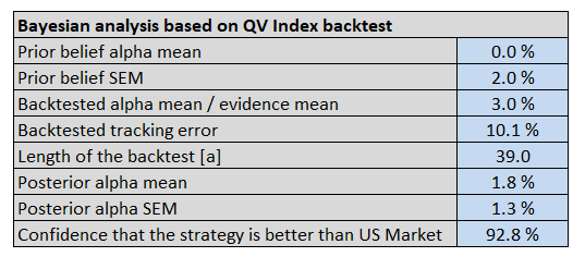
The table & graph below show the inputs and outputs of the Bayesian inference:
Some quick background on each component:
- Prior alpha mean: 0%, in line with EMH.
- Prior belief standard error: 2%, which assumes there is some noise around the EMH.
- Backtested alpha mean: 3%, which assumes a 50% haircut to the 6% alpha estimate on the QV Index (Net) from 1974 to 2012.
- Backtest tracking error: Tracking error between the QV Index (Net) and the US Market
- Length of the backtest: Expressed in years(5)
- Posterior alpha mean: http://www.ams.sunysb.edu/~zhu/ams570/Bayesian_Normal.pdf (see the bottom of page 4)
- Posterior alpha SEM: http://www.ams.sunysb.edu/~zhu/ams570/Bayesian_Normal.pdf (see the bottom of page 4)
- Strategy Confidence: See Normdist discussion above with posterior mean/SEM inserted in the function
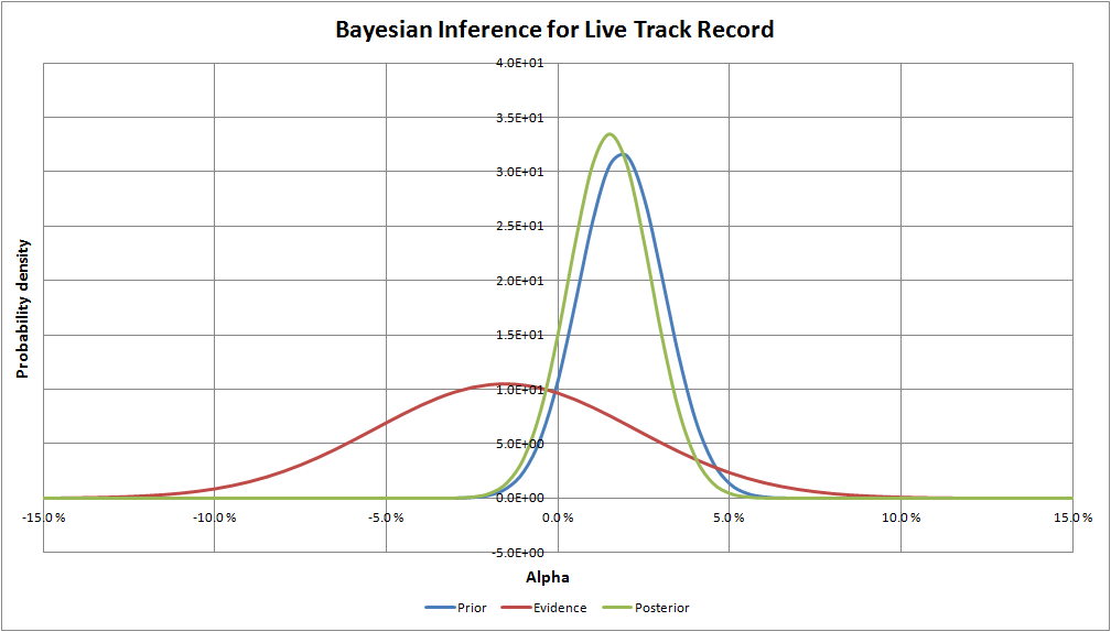
The probability distributions in the graph below represent the beliefs of the actual alpha for the QV Index (Net):
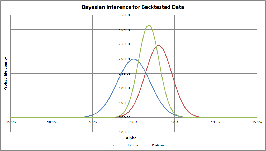
As expected, the posterior distribution lies between the prior and the evidence in the graph. Both, the prior and the evidence, contributed to the posterior view on what to expect from QV. Since we are in this case expressing the uncertainties with normal distributions, Bayesian inference formulas are simple enough to work with a spreadsheet program.
(6)To conclude, our posterior distribution of alpha is defined by an expected value of 1.8% and SEM of 1.3%. Equivalent to 92.8% confidence that the QV index outperforms it’s passive benchmark over the long term. The posterior (investment conviction) we just defined is a very important piece of information for rational decision-making. We can now look at the “out of sample” evidence from 2013 to 2017 and update our beliefs with respect to the expected QV Index (Net) distribution.
Using Bayesian Analysis to Evaluate New Information/Evidence
Okay, so after conducting the analysis above, when we were sitting in December 31, 2012 trying to figure out what do to with our money, we went with an investment in the QV Index strategy.
Fast forward five years. Underperformance — ugg!
Time to sell and switch to another strategy? Possibly, but let’s try and make a rational assessment via Bayesian analysis.
To conduct this analysis, we’ll simply take our previous posterior as our new prior and we’ll incorporate the information we’ve gleaned from the past 5 years. Earlier, we analyzed the new evidence (live track record) in the “The Frequentist Approach of Evaluating Track Records” section. We got rid of the QV strategy using that approach.
With the Bayesian approach, we crunch the data and update our beliefs.
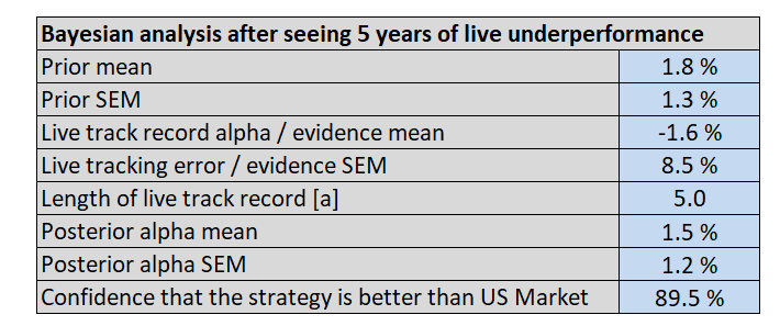
The Bayesian inference graph below makes it obvious that the new confidence level (89.5% versus 92.8%) is driven by the prior versus the new evidence. This makes sense because 5-years of data from a noisy process is usually too short to make confident conclusions, whereas, the prior probability distribution was formed based on an initial efficient market hypothesis prior and a 39-year backtest. As a result, the new data from the 5-year live out-of-sample index track record has an only minor impact on expectations of the actual alpha of QV index (1.8% before seeing the live track record and 1.5% after).
To summarize the case study, the Bayesian decision-maker had an initial conviction in choosing his investment, the QV index. But after seeing five long years of underperformance, he rationally updated his beliefs in the light of this new information. The result of the analysis was that the 5-year track record had only a minor impact on his beliefs on what to expect of his investment. So ultimately his conclusion was that the five years of underperformance most likely happened only because of bad luck, not because of wrong initial investment decision. This is completely the opposite conclusion than the frequentist decision-maker took out of his track record analysis. The reason for the disparity is that frequentists don’t have — or even care — about the prior beliefs. However, in this case, the prior turns out to be a very important piece of information for the decision-maker and for his/her conclusions. A natural question all investors should ask, is “What is your prior when you look at a track record?” The answer to this question will help drive decision-making in the future.
Conclusions
Bayesian inference is just one of the many analysis tools available to assess an ongoing investment decision. One of the nice things about Bayesian decision-making is that the framework can transparently quantify one’s subjective decision-making process. My experience is that Bayesian methods are not widely adopted, maybe partly because the prior is misunderstood and partly because the related mathematics is considered difficult. The fact that priors are subjective, does not mean that hard data analysis methods or models cannot be applied when expressing one’s view on investment decisions or on any other subject for that matter. And when it comes to math, only two simple formulas are needed if one is working with normal distributions (see references).
Editor’s note: Alpha Architect will be building a Bayesian analysis toolkit in the future to help investors make better decisions. Stay tuned!
References[+]
| ↑1 | Index data access can be requested here. Wes and the team are happy to share with other researchers and investors. |
|---|---|
| ↑2 | Philosophical Economics has a good overview). |
| ↑3 | I’ve actually seen this used a couple of times in engineering. One example is sequential Bayesian analysis for fatigue testing. In that scenario, you have some expected material strength based on material standards (prior). Hence, when you are testing the same quantity yourself it probably makes sense to start from the prior and then update your beliefs when new material test data becomes available. But in applications, most engineers do what most people do–they ignore the prior. |
| ↑4 | Feel free to use your own prior and conduct the analysis. |
| ↑5 | Sequential Bayesian updating is equivalent if new data is added to the evidence OR old estimation is taken as a prior and only the new data is put to the evidence. Math proof: http://www.stats.ox.ac.uk/~steffen/teaching/bs2HT9/kalman.pdf |
| ↑6 | The formulas to form a Bayesian posterior distribution from normally distributed prior and evidence. The posterior distribution is defined by expected value µp and standard error of the mean σp. Respectively, expected value and standard error of the mean are µ0 and σ0 for the prior distribution. The evidence, on the other hand, is often defined a bit differently in terms of parameters. µe is the expected value as for the other two but now the uncertainty is defined by the number of samples n and by standard deviation σe. The number of samples is equivalent to the number of years of data when analyzing investment track records. Annual period choice scales the standard deviation (volatility) proportional to the square root of time, as it should.
σp2 = (1/σ02 + n/σe2)-1 (1) µp = σp2 [µ0/σ02 + (n*µe)/σe2] (2) |
About the Author: Joni Keski-Rahkonen
—
Important Disclosures
For informational and educational purposes only and should not be construed as specific investment, accounting, legal, or tax advice. Certain information is deemed to be reliable, but its accuracy and completeness cannot be guaranteed. Third party information may become outdated or otherwise superseded without notice. Neither the Securities and Exchange Commission (SEC) nor any other federal or state agency has approved, determined the accuracy, or confirmed the adequacy of this article.
The views and opinions expressed herein are those of the author and do not necessarily reflect the views of Alpha Architect, its affiliates or its employees. Our full disclosures are available here. Definitions of common statistics used in our analysis are available here (towards the bottom).
Join thousands of other readers and subscribe to our blog.