The 52 Week High and the Q-Factor Investment Model

In the past, we have examined the following two topics: (1) stock performance & the 52-week high and (2) the investment CAPM.

When examining the performance of stocks relative to their respective 52-week high (highlighted by us here), the authors (George and Hwang) find the following:

When coupled with a stock’s current price, a readily available piece of information—the 52-week high price–explains a large portion of the profits from momentum investing. Nearness to the 52-week high dominates and improves upon the forecasting power of past returns (both individual and industry returns) for future returns.

In short, buying stocks close to their 52-week high, and selling stocks close to their 52-week low is a momentum strategy. We examine this in detail in the appendix of our Quantitative Momentum book and find that while the 52-week high screen is an alternative way to form a momentum portfolio, we still prefer to use total-return momentum because the 52-week high signal is not robust to small alterations (e.g., holding period).

However, one thing is clear–using a 52-week high screen clearly gives an indication of the current price relative to its past prices. At some level, this is an indication of what the market believes in the stock (both in the past and the future).

We also examined the investment CAPM model via a long interview with Lu Zhang.

Here is a good paper (by Lu) where his introduction explains what he is doing:

Intuitively, the consumption CAPM, which is derived from the first principle of consumption, connects expected returns to consumption betas. The consumption CAPM predicts that consumption betas are sufficient statistics for expected returns. Once consumption betas are controlled for, characteristics should not affect the cross section of expected returns. This prediction is the organising framework for the bulk of empirical finance and capital markets research in accounting.

The investment CAPM, which is derived from the first principle of investment, connects expected returns to characteristics. It predicts that characteristics are sufficient statistics for expected returns. Once characteristics are controlled for, consumption betas should not affect expected returns. As such, the consumption CAPM and the classic CAPM as its special case miss what neoclassical economics has to say about the cross section of expected returns from the investment side altogether. Derived from the two-period manager’s problem, the investment CAPM is the dual proposition to the classic CAPM, which is in turn derived from a two-period investor’s problem.

So Lu changed the assumption on who is maximizing (a company, not a household), and comes up with profitability and investment as the two main factors. His Q-factor model has four factors: the Market, Size, Profitability, and Investment. In another paper we covered (similar idea), called Replicating Anomalies, Lu finds that the Investment CAPM, and its respective Q-factor model, generally do a better job of explaining the cross-section of stocks than the current asset-pricing models (FF 3-factor, Carhart 4-factor, and FF 5-factor).⁽¹⁾

So why are we re-visiting old post and topics?

There is a new forthcoming JFE paper, titled “The 52-Week High, q Theory and the Cross-Section of Stock Returns,” by George, Hwang, and Li, that examines the two topics discussed above– (1) the 52-week high and (2) the q-factor model.

Below we dig into the paper.

Does the Q-factor model better capture the 52-week high anomaly?

The original 52-week high paper by George and Hwang (2004) finds the following price-to-high (PTH) anomaly: firms with stock prices nearest to their 52-week highs (high-PTH firms) earn higher factor-adjusted returns on average than firms whose stock prices are farthest from their 52-week highs (low-PTH firms).

So how well does the Q-factor model capture the PTH anomaly?

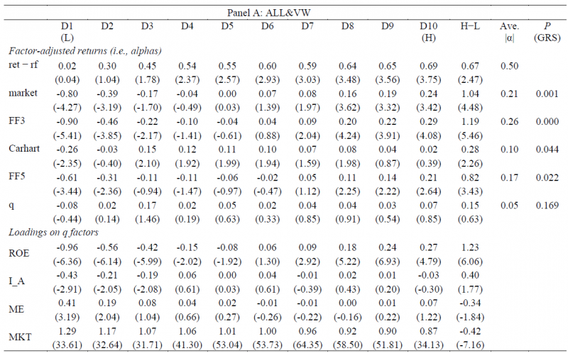
The paper examines this in Table 1, by regressing the deciles and L/S portfolio formed on the price-to-high (PTH) variable. The results are shown below to Panel A, which includes all stocks and value-weights the portfolios:

The results are hypothetical results and are NOT an indicator of future results and do NOT represent returns that any investor actually attained. Indexes are unmanaged, do not reflect management or trading fees, and one cannot invest directly in an index.

Going from left to right, the decile returns are shown, with D1 being the decile of stocks furthest from the 52-week high, and D10 being the decile of stocks closest to the 52-week high. The H-L portfolio examines the L/S to the portfolio that goes long Decile 10 and short Decile 1.

Moving from the top to the bottom, the table examines the raw returns above the risk-free rate (ret-fr), as well as the alphas to five different factor models: (1) the market model, (2) the FF 3-factor model, (3) the Carhart 4-factor model, (4) the FF 5-factor model, and (5) the q-factor model.

As is shown above, the decile returns to the first 4 models, save the Q-factor model, have significant alphas (either negative or positive). Examining the L/S portfolios, the first 4-models generate a highly significant L/S portfolio return, while the q-factor model yields an insignificant alpha. The last column gives the p-value for the GRS test, whose null hypothesis is that the alphas are jointly zero across the deciles. As is shown above, examining Panel A, which includes all stocks and value-weights the portfolios, the first 4 factor models are rejected by the GRS test (p-values < 0.05), whereas the q-factor model is not rejected.

Last, we notice that there is a statistically significant loading on the ROE factor (t-stat of 6.06 for the H-L portfolio). Thus, it appears that the q-factor picks up the PTH anomaly through the ROE factor (as a reminder, the ROE factor is monthly rebalanced using quarterly updated data).

But what about alternative weighting schemes, and do micro-caps matter?

Panel B of Table 1 (not shown here) excludes micro-cap stocks and equal-weights the portfolio. It finds that the q-factor model is rejected according to the GRS test while the L/S portfolio is statistically insignificant under the q-factor model. For the other factor models, the L/S portfolios generate statistically significant L/S alphas. The results are generally similar in Panel C where the authors change the holding period from 6 months to either 1 or 12 months.

So the results lead to the authors’ conclusion:

These results suggest that the q-factor model captures the PTH anomaly better than all the other factor models that we consider.

The authors go on to highlight how the q-factor model performs when completing a double sort on (1) PTH and (2) Asset growth:

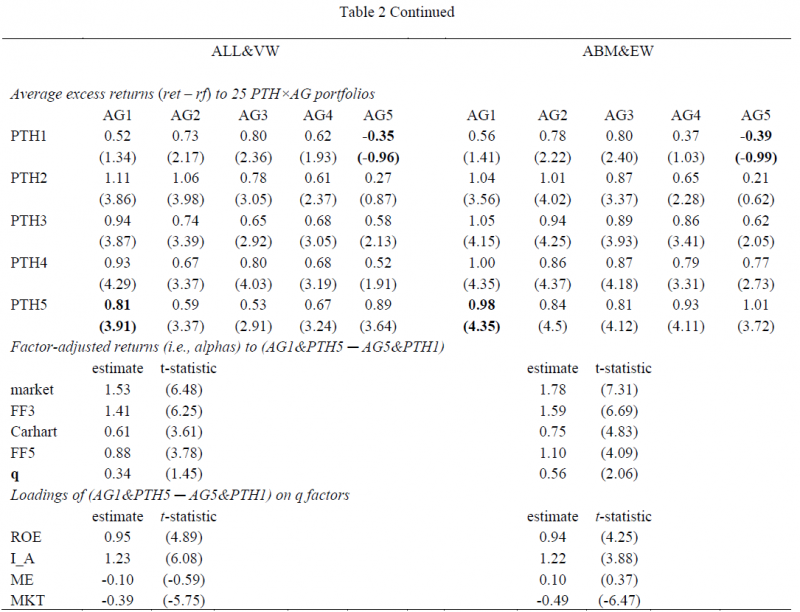
[the] hypothesis is that stocks with high (low) PTH and low (high) asset growth earn very high (low) future returns, and that these extreme returns are better captured by the q-factor model than by the other models.

The results are shown in Table 2 below:

The results are hypothetical results and are NOT an indicator of future results and do NOT represent returns that any investor actually attained. Indexes are unmanaged, do not reflect management or trading fees, and one cannot invest directly in an index.

As is shown above, firms that are closest to the 52-week high (PTH5) with low asset growth (AG1) have the highest average excess returns–this is documented by the 0.81% average monthly excess return for the all-stock, value-weighted portfolio. Alternatively, stocks that are the furthest from their 52-week high (PTH1) with high asset growth (AG5) have the lowest average excess returns–this is documented by the -0.35% average monthly excess return for the all-stock, value-weighted portfolio.

Next, the paper examines the long short returns to the “extreme” portfolios–(1) go long PTH5 & AG1 portfolio and (2) go short the PTH1 & AG5 portfolio. When examining the alpha from the factor models, one notices that for the first four models, there is a statistically significant alpha. However, for the q-factor model, the alpha is insignificant. Thus, the q-factor model does the best job of explaining the spreads in this L/S portfolio.  Not surprisingly, this is mostly due to high loadings on the ROE (Profitability) and Investment factors.

So does the PTH variable help to better explain the cross-section of stock returns?

The authors examine this question below.

Does adding PTH to the Q-Factor model help explain the cross-section of stock returns?

As mentioned in the Replicating Anomalies paper, while the q-factor model does a better job of explaining the cross-section of stock returns, there are still some anomalies that exist. So does adding information from the PTH variable help to better explain the cross-section?

The authors find the following:

HXZ (2015) find that the q-factor model outperforms FF3 and Carhart models in capturing a wide range of anomalies, but underperforms them in capturing these two anomalies: the operating accrual (OA) anomaly and the R&D-to-market (RD/M) anomaly. It is possible that these two anomalies are consistent with the investment CAPM, and the reason the q-factor model fails in capturing them is because OA and RD/M contain information about expected investment growth, which is not captured well by the ROE factor in the q model.

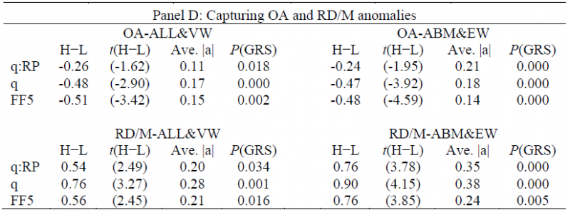
The authors first find a link between the PTH variable and expected investment growth (Table 3). Next, the authors find (in Table 4, Panel D) that by adjusting the ROE factor to include price-level variables (i.e. closeness to 52-week high), they can better explain two of the anomalies in the q-factor model– operating accruals and R&D-to-market.

The results are shown below:

The results are hypothetical results and are NOT an indicator of future results and do NOT represent returns that any investor actually attained. Indexes are unmanaged, do not reflect management or trading fees, and one cannot invest directly in an index.

Examining the table above, we notice that for the operating accrual (OA) and R&D/market (RD/M) anomalies, the augmented q-factor model (q:RP above) does a better job of explaining these anomalies, due to the lower (and sometimes insignificant) alpha estimates from the augmented q-factor model.

Conclusion

At a high level, this paper finds a few items:

1. Examining the nearness to the 52-week high variable (a form of momentum), the q-factor model is better than other models at picking up this variable in the cross-section.
2. Firms with high momentum (close to 52-week high) and low asset growth perform the best.
3. Augmenting the ROE factor (from the q-factor model) by adding a price variable (nearness to 52-week high) enhances the model’s ability to explain the cross-section of stock returns.

I wonder if this is the first of many papers that will show enhancements to the q-factor model, similar to how the FF 3-factor model was enhanced over the years. (We already know Lu Zhang and his team are enhancing their q-factor model with an expected growth factor, which may explain the PTH factor. Here is their Q^5 paper)

Let us know what you think …

The 52-Week High, q Theory and the Cross-Section of Stock Returns

• Thomas J. George, Chuan-Yang Hwang, and Yuan Li
• A version of the paper can be found here.
• Want a summary of academic papers with alpha? Check out our Academic Research Recap Category.

Abstract:

Hou, Xue and Zhang’s (2015) q-factor model outperforms other factor models in capturing the PTH (the ratio of current price to 52-week high price) anomaly: High-PTH stocks earn high future returns. PTH’s relations with future profitability and future investment growth are both significantly positive, and they mirror PTH’s relation with future returns in the cross-section and by time horizons. Incorporating the information about future investment growth contained in price level variables (e.g., PTH) helps the q factors to capture better those anomalies rooted in future investment growth. Together, these results suggest that the PTH anomaly is consistent with the investment CAPM.