When it comes to predicting long-term equity returns, several well-known indicators come to mind—for example, the CAPE ratio, Tobin’s Q, and Market Cap to GDP, to name a few.
Yet there is another indicator without nearly as high of a profile that has outperformed the aforementioned indicators significantly when it comes to both forecasting and tactical asset allocation.
That indicator, known as the Aggregate (or Average) Investor Allocation to Equities (AIAE), was developed by the pseudonymous financial pundit, Jesse Livermore, and published on his blog in 2013.
In an essay titled, “The Single Greatest Predictor of Future Stock Market Returns,” Livermore makes the case that the primary driver of long-term equity returns is not valuation, but rather the supply of equities relative to the combined supply of bonds and cash.
Accordingly, the AIAE is computed by taking the total market value of equities and dividing by the sum of a) the total market value of equities, b) the total market value of bonds, and c) the total amount of cash available to investors (i.e., that in circulation plus bank deposits):
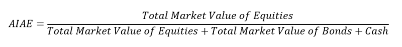
This ratio gives the market-wide allocation to equities (or, equivalently, the average investor allocation to equities weighted by portfolio size). (Note that every share of stock, every bond, and every unit of cash in existence must be held in some portfolio somewhere at all times.)
Livermore explains that, in practice, the total market value of bonds plus cash can be estimated by the total liabilities held by the five classes of economic borrowers: Households, Non-Financial Corporations, State and Local Governments, the Federal Government, and the Rest of the World.
This follows from the fact that if these entities borrow directly from investors, new bonds are created. Whereas, if they borrow directly from banks, new bank deposits (cash) are created.
As the economy grows, the supply of bonds and cash steadily increases. Historically, the rate of increase of the supply of bonds and cash has been about 7.5% per annum. Consequently, if the market portfolio is to maintain the same allocation to equities, the supply of equities must increase at the exact same rate.
The supply of equities can increase either by new equity issuance or by price increases. Historically, net new equity issuance has been negligible (with issuances being offset by buybacks and acquisitions). Thus, in order for equities not to become an ever-smaller portion of the average investor’s portfolio, the price of stocks must rise over the long-term.
While we often hear that stock prices follow earnings, in the 1980s earnings fell slightly from the beginning of the decade to the end of the decade, yet stocks rose at an annualized rate of 17% during that time. How could this be?
Well, at the beginning of the decade the average investor’s portfolio had a 25% allocation to equities. During the decade, the supply of bonds and cash rose strongly. If the price of equities had not risen, the average investor’s allocation to equities would have fallen to a mere 13% (as the supply of cash and bonds grew). Thus, equities had no choice but to rise despite the fall in earnings.
Livermore proposes a new framework for how we view the components of the equity market’s total return. Instead of viewing the total return in a classic way, namely:
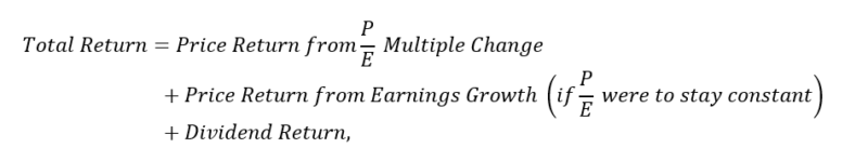
he suggests we should instead view the components as:
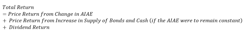
As Livermore states:
“This way of thinking about stock market returns accounts for relevant supply-demand dynamics that pure valuation models leave out. That may be one of the reasons why it better correlates with actual historical outcomes than pure valuation models.”
In a subsequent essay titled “Valuation and Stock Market Returns: Adventures in Curve Fitting,” (1) Livermore throws a bit of cold water on all indicators (including the AIAE) used to “forecast” future stock returns. He notes:
“[L]ooking backwards and fitting valuation metrics to precise returns so as to come up with a precise estimate is not a productive exercise. Unless the ensuing “value v. return” charts are rigorously and extensively tested out of sample (without the chart-maker already knowing the answer, and being able to spend time “tweaking” out a visually-pleasing hindsight fit that takes advantage of happenstance coincidences in market history), their predictions should be ignored, or at least taken very lightly, as an extremely general comment about the future.”
With respect to this point, in a paper titled, ‘Towards a Better Fed Model,’ (2) we take up the task of testing the AIAE—as well as six other indicators—using walk-forward regressions to see if it does in fact merit the title “The Single Greatest Predictor of Future Stock Market Returns.”
LONG-TERM EQUITY RETURN FORECASTS
The indicators we examine include:
- AIAE
- CAPE (3)
- Tobin’s Q (QRATIO) (4)
- Market Value to GDP (MC/GDP) (5)
- Market Value to Adjusted Gross Value Added of Non-Financial Corporations (MC/AGVANF) (6)
- Market Cap to Household and Non-Profits Total Assets (MC/HHNPTA) (7)
- Household and Non-Profit Equities to GDP (HHNPEQ/GDP) (8)
To make a long story short, the AIAE does indeed produce the best ex-ante long-term stock forecasts.
Figure 1 shows the mean and maximum absolute deviations between the various indicators’ ex-ante 10-year annualized return forecasts and the subsequent actual 10-year annualized returns from 1970-2020. Here we see the AIAE has had both the lowest mean and maximum absolute deviations between its forecasts and the actual realized returns.
Figure 2 shows the same quantities from the year 2000 onward. From Figure 2 we see that the AIAE’s predictions have gotten even better over the last two decades.
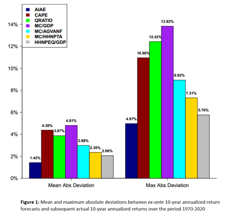
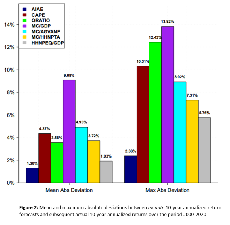
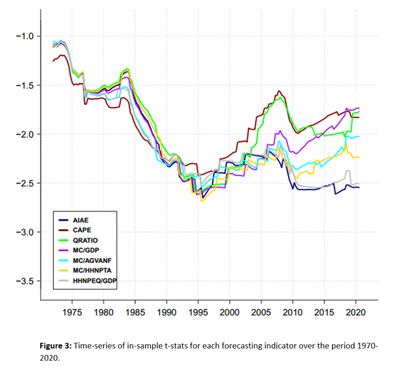
Figure 3 shows the evolving in-sample t-stats of the indicators’ regression coefficient (found using an expanding window walk-forward regression using a method that accounts for the overlap in the data (9)). With the exception of the AIAE and HHNPEQ/GDP, the statistical significance of the other indicators has gotten notably worse since the mid-90s.
TACTICAL ASSET ALLOCATION
In addition to evaluating the indicators’ forecasting ability, we also examined their effectiveness within a tactical asset allocation framework. Where again we observed the AIAE to deliver to the most consistently solid overall performance—measured across the full time period and various subperiods.
We created tactical asset allocation strategies for each of the indicators listed above by taking their 10-year equity return forecast and subtracting the 10-year bond yield (which, according to John Bogle, is the single best predictor of 10-year bond returns (10)) to generate an expected equity risk premium.
Next, we computed modified z-scores of the expected risk premium by subtracting from it the median value of actual 10-year equity risk premia (10-year equity returns minus 10-year bond returns) from the preceding 120 months and dividing by their standard deviation.
We then allocated to U.S. equities or an aggregate bond index based on the following algorithm:
- If the modified z-score was greater than 1, invest 100% in equities.
- If the modified z-score was less than -1, invest 0% in equities.
- In between -1 and 1, use linear interpolation (thus, a z-score of 0 would generate an equity allocation of 50% and so on).
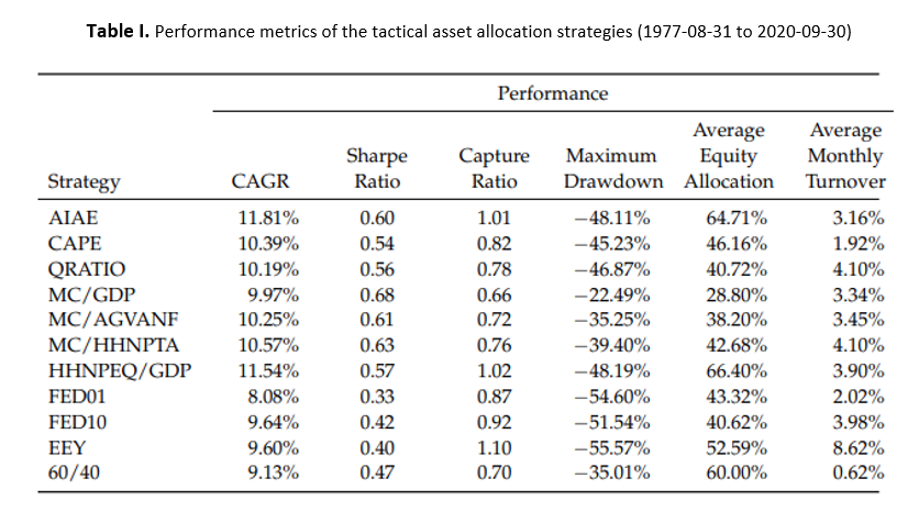
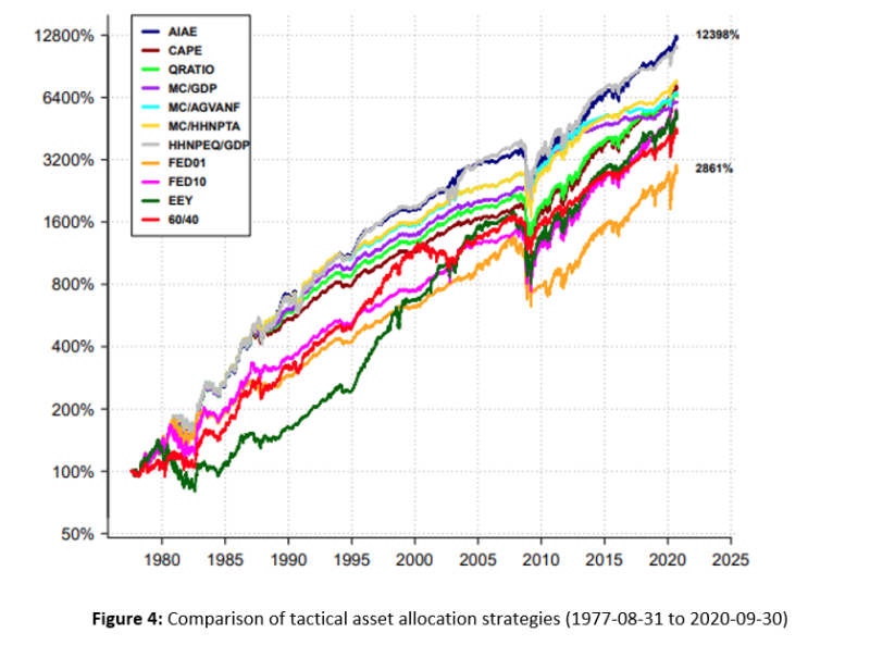
Table I shows the full historical performance of the indicators along with four other strategies (a Fed Model(11) using trailing 1-year earnings data (FED01), a Fed Model using trailing 10-year earnings data (FED10), the excess earnings yield model (EEY) (12), and a 60/40). Figure 4 shows their respective equity curves.
From Table I we can see that the AIAE slightly edges out the HHNPEQ/GDP metric for the highest total return. The AIAE also has the highest Sharpe ratio of all strategies that have greater than 50% average allocation to equities.
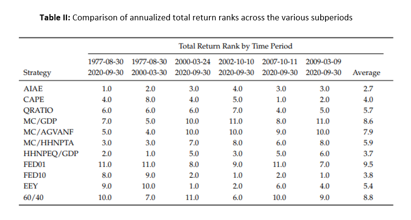
We also examine the performance across various subperiods of the total time history. Table II shows the rank of the total return across each subperiod for each strategy—from which we see that the AIAE had the best average rank across the subperiods (finishing 1st, 2nd, 3rd, 4th, 3rd, and 3rd across the six periods examined). The next best strategy, HHNPEQ/GDP, had ranks of 2nd, 1st, 5th, 3rd, 5th, and 6th.
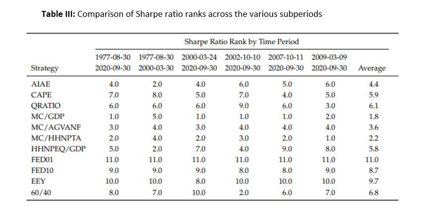
Table III shows the average Sharpe ratio rank across the subperiods. The AIAE had the highest rank among all strategies that allocated more to equities than bonds, on average, across the subperiods. (Note that MC/GDP, MC/AGVANF, and MC/HHNPTA appeared to systematically underestimate the equity risk premium and thus placed most of their assets in bonds—leading to lower returns, but higher Sharpe ratios.)
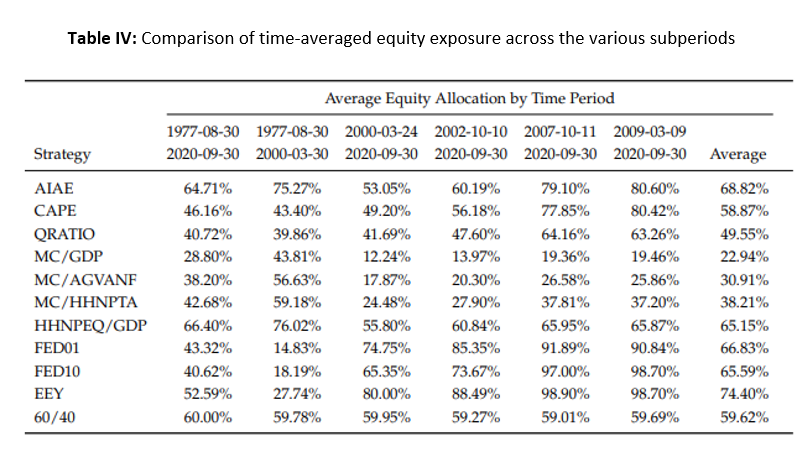
Table IV shows the average equity exposure across the subperiods. Other than MC/GDP, MC/AGVANF, and MC/HHNPTA, the strategies averaged between 50% and 75% equity exposure.
As is evident, the AIAE was not light-years better than its competitors with respect to tactical asset allocation. But it did appear to be the most reliable—generating the most consistently high performance across time (likely a function of its generally superior forecasting accuracy). In contrast, many of its competitors tended to do very well in certain subperiods and very poorly in others.
THE AIAE and MARKET DYNAMICS
One notable characteristic of the AIAE is that its computation involves only market-based, i.e., endogenous, quantities—the market value of equities, the market value of bonds, and the supply of cash. In contrast, the other indicators involve exogenous quantities—earnings, book value, GDP, GVA, etc.
As a result, the AIAE appears able to provide insight on equity market dynamics that the other indicators cannot. For example, recent history has shown us how anticipatory changes in the supply of bonds and cash can affect equity markets.
During the Great Recession, investors feared widespread insolvencies. Such insolvencies would have reduced the supply of bonds, causing the aggregate market portfolio to be overallocated to equities relative to pre-crisis preferences. As a consequence, investors repriced equities downward to regain an equilibrium (and perhaps overshot what was reasonable due to the prevailing “doom and gloom” environment).
The Great Recession bear market stopped and reversed course only when the U.S. Financial Accounting Standards Board (FASB) changed the rules to allow companies to mark their portfolios to model rather than to market (13). This change eliminated the specter of mass insolvencies (which stabilized the denominator of the AIAE). Suddenly, the market-wide portfolio became significantly underinvested in equities relative to pre-crisis preferences. Equities bottomed and began their long journey higher.
More recently, during the COVID-19 panic of March 2020, investors again feared widespread insolvencies—possibly on a scale greater than the Great Recession. As before, such insolvencies would have left investors’ portfolios overexposed to equities relative to pre-crisis preferences. The resulting equity market selloff was fast and steep—the S&P 500 lost 35% in 23 trading days.
But when the Federal Reserve announced on March 23, 2020, it would be buying corporate bonds as needed to calm markets, the prospect of investors being overexposed to equities was no longer a concern (14). By replacing the bonds in investors’ portfolios with cash, the Federal Reserve stabilized the denominator of the AIAE.
Indeed, investors now found themselves substantially underexposed to equities relative to their pre-crisis preferences. Equities bottomed on the day of the Fed announcement and went on to make new all-time highs by the summer of 2020.
As one can see from these examples, the structure of the AIAE sheds light on how equities are likely to react given a change (or stabilization) in the supply of bonds and cash. In contrast, valuation measures based on earnings or nominal GDP (both of which were seriously impaired during both the Great Recession and the COVID-19 crisis) do not seem to provide the same level of insight.
Instead, one observes such valuation measures becoming more and more “overvalued” as the equity market rises, in spite of continued economic impairment. The natural inference, then, is that asset-supply dynamics are a much more primal determinant of equity market behavior than traditional measures of value.
CURRENT FORECASTS
As of April 26, 2021, the AIAE is forecasting 1.05% annualized over the next 10 years for U.S. equities. The 10-year yield is at 1.57%. Thus, the expected equity risk premium is -52 basis points. (Note that the expected equity risk premium was negative for over 4 years(!) during the run-up to the dotcom market top and for two months prior to the 2007 market top.)
When one considers that the dividend yield on the S&P 500 is approximately 2%, the annualized price return of the U.S. equity market is likely to be slightly negative (from these levels) over the next 10 years. Thus, it is quite possible we may see the S&P 500 somewhere between 3500 and 4000 in 2031.
CONCLUSION
While rarely mentioned in discussions of equity forecasting indicators, the AIAE does appear to be the single greatest predictor of long-term equity returns currently in the public domain.
References[+]
| ↑1 | Livermore, Jesse, 2013, Valuation and Stock Market Returns: Adventures in Curve Fitting, https://www.philosophicaleconomics.com/2013/12/valuation-and-returns-adventures-in-curve-fitting/ |
|---|---|
| ↑2 | Micaletti, Raymond, 2020, Towards a Better Fed Model, SSRN Electronic Journal, URL: https://ssrn.com/abstract=3704963. |
| ↑3 | Campbell, John Y., and Robert J. Shiller, 1987, Stock prices, earnings, and expected dividends, The Journal of Finance 43, 661–676. |
| ↑4 | Tobin, James, and W.C. Brainard, 1977, Economic Progress, Private Values and Public Policy. |
| ↑5 | Buffett, Warren, and Carol Loomis, 2001, Warren buffett on the stock market, https://archive.fortune.com/magazines/fortune/fortune_archive/2001/12/10/ 314691/index.htm |
| ↑6 | Hussman, John P., 2015, The new era is an old story (and introducing market cap/gva), http://www.hussmanfunds.com/wmc/wmc150518.htm. |
| ↑7 | Vallee, Teddy, 2020, https://twitter.com/TeddyVallee/status/1262752665571692551. |
| ↑8 | Vallee, Teddy, 2020, https://twitter.com/TeddyVallee/status/1262752665571692551. |
| ↑9 | Britten-Jones, Mark, Anthony Neuberger, and Ingmar Nolte, 2011, Improved inference in regression with overlapping observation, Journal of Business Finance & Accounting 38, 657–683. |
| ↑10 | Gay, Chrisk, 2014, How to predict the next decade’s bond returns, URL: wsj.com/articles/how-to-predict-the-next-decades-bond-returns-1393871478. |
| ↑11 | Yardeni, Ed, 1997, Fed’s stock market model finds overvaluation, US Equity Research Deutsche Morgan Grenfell. |
| ↑12 | Salomons, Roelof, 2004, A tactical implication of predictability: Fighting the fed model, SSRN Electronic Journal, URL:https://ssrn.com/abstract=517322. |
| ↑13 | Halbert, Gary, 2018, Did “mark-to-market” rules cause the financial crisis?, https://www.advisorperspectives.com/commentaries/2018/09/18/did-markto-market-rules-cause-the-financial-crisis.. |
| ↑14 | Smialek, Jeanna, 2020, The fed goes all-in with an unlimited bond-buying plan, https://www. nytimes.com/2020/03/23/business/economy/coronavirus-fed-bond-buying.html. |
About the Author: Raymond Micaletti
—
Important Disclosures
For informational and educational purposes only and should not be construed as specific investment, accounting, legal, or tax advice. Certain information is deemed to be reliable, but its accuracy and completeness cannot be guaranteed. Third party information may become outdated or otherwise superseded without notice. Neither the Securities and Exchange Commission (SEC) nor any other federal or state agency has approved, determined the accuracy, or confirmed the adequacy of this article.
The views and opinions expressed herein are those of the author and do not necessarily reflect the views of Alpha Architect, its affiliates or its employees. Our full disclosures are available here. Definitions of common statistics used in our analysis are available here (towards the bottom).
Join thousands of other readers and subscribe to our blog.