Trend-Following Filters – Part 8

1. Introduction

Regression analysis is a statistical method used to estimate and model the relation between a dependent variable and one or more independent variables. The dependent variable, also called the observation, is the variable being explained or predicted. The Independent variables are used to explain or predict the dependent variable. In economics, regression analysis is used, for example, to measure relationships between macroeconomic variables such as GDP, inflation, unemployment, interest rates, money supply, etc. In finance, it is the basis of various factor models, such as the Capital Asset Pricing Model (CAPM) and the Fama-French and the Carhart models. Detailed discussion of regression analysis and its uses can be found in numerous textbooks and course lectures, such as [1] and [2].

Regression is also used in time series analysis. In trading, for example, there are several technical analysis market indicators based on regression that are used to identify trends in financial time series, e.g., Linear Regression Slope [3] and Time Series Forecast [4]. This article describes digital filters derived from time series regression models that can be used as technical analysis tools. The filters are analyzed from a digital signal processing (DSP) frequency domain perspective to illustrate their properties. Example charts of the filters applied to the S&P 500 index are also included.

Some familiarity with DSP concepts is assumed. Refer to [5] for more detailed discussion of various DSP-related terminology and topics, including frequency, period, types of digital filters such as low pass and bandpass filters, frequency response, difference equations, cutoff frequency, center frequency, etc.

2. Time Series Regression Models and Least Squares

In time series regression models, the independent variables are based on time, and the dependent variable is a series of corresponding data points organized in time sequence order. For example, a stock chart displays a time series of prices, where the independent variable, time, is represented on the horizontal x-axis as a series of discrete uniform time steps and the dependent variable, the price at each time step, is represented on the vertical y-axis. The time step intervals can be hourly, daily, weekly, monthly, etc.

The goal of regression analysis is to estimate the model that most closely fits the relation between the dependent and independent variables. A regression model is a mathematical equation, the general form of which is:

where

• y = dependent variable (observation),
• k+1 = number of independent variables and model parameters,
• x_k = independent variables where x₀ = 1,
• β_k = model parameters, and
• ε = estimation error.

The regression modeling process involves determining the number and type of independent variables involved and the corresponding model parameters. In the case of time series regression, the number and type of independent variables can, for example, be based on an assumed underlying time series process. Once established, the next step is to estimate the model parameters that best fit the independent variables to the dependent variable observations.

For a given set of independent variables x_k and parameters β_k, the regression model can be used to predict the corresponding dependent variable y. The regression model prediction y` is:

The prediction error e is the difference between the actual value y and the prediction y`:

A common approach to determine the model parameters β₀, β₁, β₂, …, β_k that best fit a set of observations is to invoke the “least squares” criterion, which seeks to find the parameters that minimize the sum of the squared errors (SSE) between the observations y_i and model predictions y`_i. For a set of N observations y₁, y₂, y₃, …, y_N, the corresponding predictions are:

The sum of squared errors SSE is:

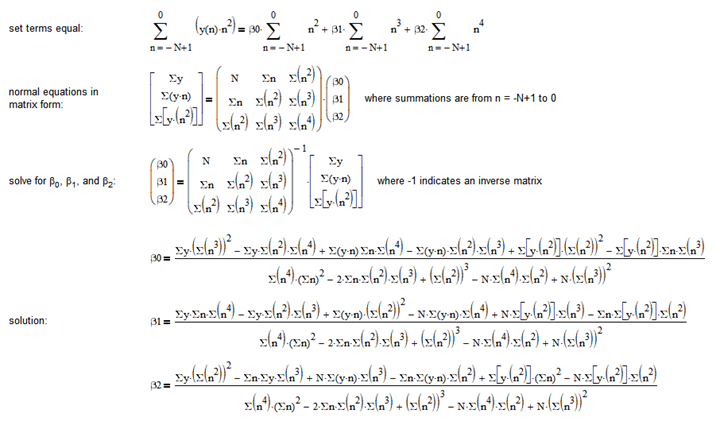
A commonly-used method to determine the parameters that minimize the SSE is to use so-called “normal equations”, which are an analytic solution to the least squares criterion. The normal equations are obtained by calculating the partial derivatives of SSE with respect to each parameter β_k and setting each one equal to zero:

Depending on the number of regression model parameters k+1, the result is a set of k+1 equations with k+1 unknowns β_k, which can be solved for β_k using matrix algebra.

3. Formulating Time Series Regression Models as Digital Filters

In this article, digital filters are derived from time series regression models. Instead of using all of the observations in a data set to fit the model, the regression models in this article use a moving or sliding window subset of the observations where the window is moved across the observations one time step at a time. Windowing allows the filter output to adapt to changes in the characteristics of the time series over time, which is particularly important in the case of financial time series, due to their volatility and non-stationarity [5].

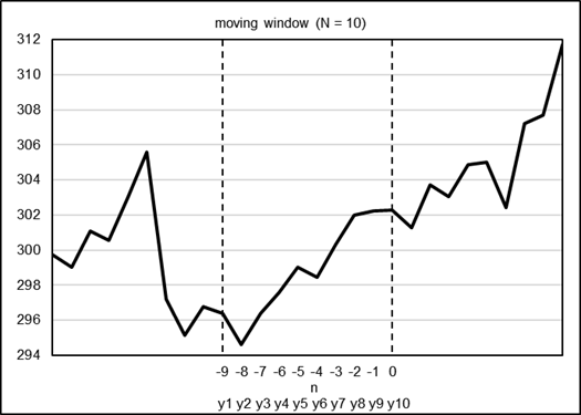
For a window length of N time steps, the time step count ranges from -N+1 to 0, where the most recent observation in the window is at 0. The example graph below illustrates a window of length N = 10, consisting of time steps n = -9, -8, -7, …, 0 which correspond to observations y₁, y₂, y₃, …, y₁₀, respectively.

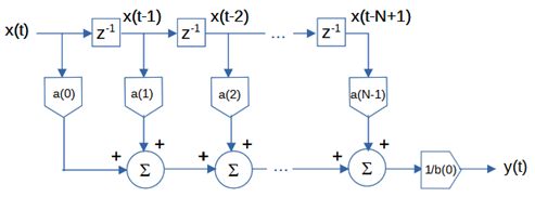
Given the form of the windowed time series regression model, the corresponding digital filter is realized as a finite impulse response (FIR) filter. A FIR filter uses only current and past input values and no past output values. The general FIR filter difference equation (also called an input-output equation) is:

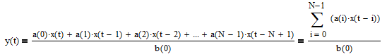
where

• y(t) = filter output at integer time t,
• N = number of filter input samples,
• x(t-i) = filter input sample at integer time t-i for i = 0, 1, 2, …, N-1,
• a(i) = filter coefficient of filter input x(t-i), and
• b(0) = filter coefficient of filter output y(t).

For the filters derived in this article, b(0) = 1.

Sections 4 through 6 and the accompanying appendices that follow show the detail derivation of the filter coefficients a(i) from windowed time series regression models that in turn are based on several different underlying time series process assumptions. In the derivations, the filter inputs x(t-i) for i = 0, 1, 2, …, N-1 correspond to the regression dependent variable observations y₁, y₂, …, y_N in the window, respectively, i.e., x(t-N+1) = y₁, x(t-N+2) = y₂, x(t-N+3) = y₃, …, x(t) = y_N. The filter coefficients are derived from the corresponding regression parameters β_k and are functions of N and i. The filter output y(t) corresponds to the most recent time step in the window and is recalculated at each time step by applying the filter coefficients to the current filter inputs in the window. As is shown, for a filter of a given length, the filter coefficients are fixed and so do not need to be recalculated at each time step, eliminating the need for repeatedly performing complex regression calculations.

Notes on the Graphs

a. Each of the following sections contains graphs of the frequency responses of the filters, using a common example length N = 10. There are two components of frequency response:

• magnitude response – the ratio of the amplitude of the filter output to the amplitude of the filter input across a range of frequencies (f), i.e., the number of cycles per time step, on the horizontal scale
• phase response – the angular shift (i.e., time delay) of the filter output relative to the filter input across the same range of frequencies, measured in degrees.

Graphs showing the magnitude response in terms of period (P), i.e., the number of time steps to complete one cycle, on the horizontal scale are also included, since period is the measurement that is most commonly used by and familiar to technical analysts. Note that P = 1/f. See [5] for additional details regarding frequency, period, and frequency response.

b. The filter coefficients are shown graphically to indicate the relative weights placed on the corresponding filter inputs.

c. Charts of the filters applied to the daily S&P 500 index for the year 2023 are also included.

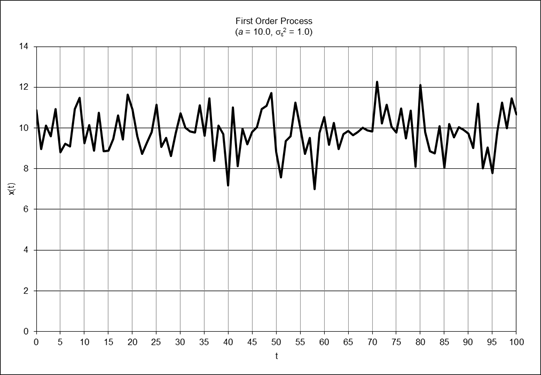
4. First Order Process Filter

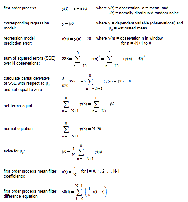
A time series based on a first order process consists of a locally constant mean a which is contaminated with random normally distributed noise ε(t) where ε(t) ~ N(0, σ_ε²):

y(t) = a + ε(t)

The following graph shows an example of a time series based on an underlying first order process:

A time series regression model based on a first order process has the form:

where y is the dependent variable and β₀ is the estimated mean. The model parameter β₀  corresponds to the coefficients of a first order process mean filter.

First Order Process Mean Filter

Appendix 1 shows the derivation of the difference equation of the first order process mean filter, which is:

where N is the number of input data points (N > 1) and x(t-i) is the filter input at integer time t-i. The first order process mean filter is a FIR low pass filter, i.e., it passes frequencies below the -3 dB (half power) cutoff frequency f_c and attenuates frequencies above the cutoff frequency. The value N determines the cutoff frequency, which is inversely proportional to N (the cutoff period P_c is proportional to N).

Note that the difference equation of this filter is equivalent to that of a moving average (MA) filter (see [5] for details of the MA filter).

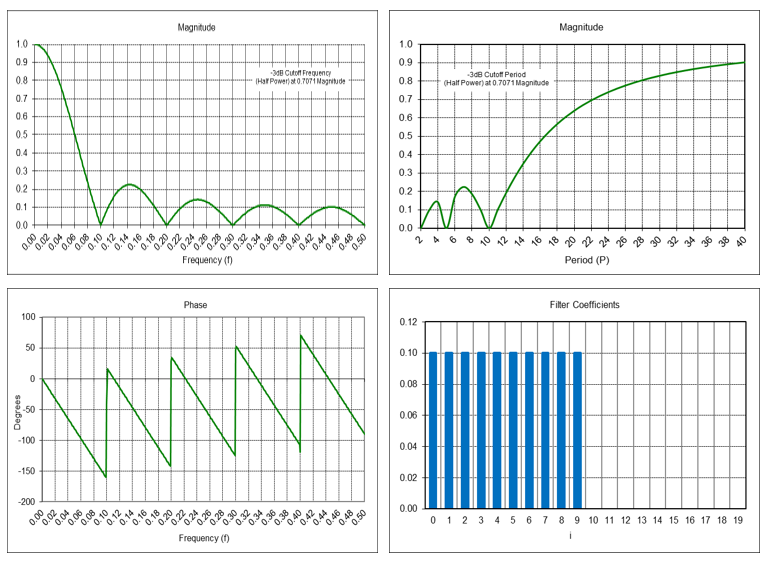
First Order Process Mean Filter Frequency Response (N = 10)

Example: First order process mean filter with length N = 10

Passes frequencies below the -3 dB cutoff frequency f_c of approximately 0.044, which corresponds to a cutoff period P_c of approximately 22.5 time samples.

First Order Process Mean Filter Example

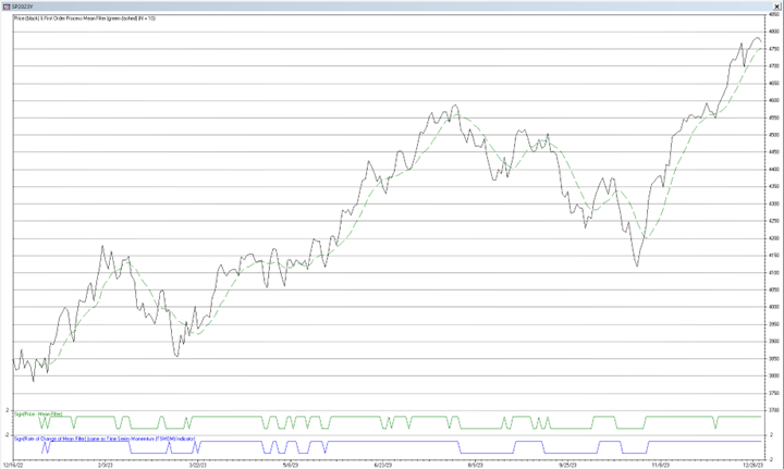
The chart below shows the first order process mean filter (green dashed line) with length N = 10 applied to the daily S&P 500 index for the year 2023.

Trading Signal Generation

A trading signal can potentially be generated when the current price crosses above (buy) or below (sell) the first order process mean filter output line. The trading signals are indicated by the line next to the bottom of the chart. Also shown at the bottom are trading signals generated by a time series momentum filter (TSMOM), a popular technical indicator which is mathematically related to the moving average (see [5] for details).

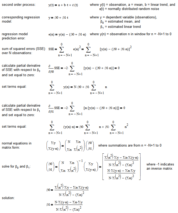
5. Second Order Process Filters

A time series based on a second order process consists of a mean a and a linear trend b which is contaminated with random normally distributed noise ε(t) where ε(t) ~ N(0, σ_ε²):

y(t) = a + b*t + ε(t)

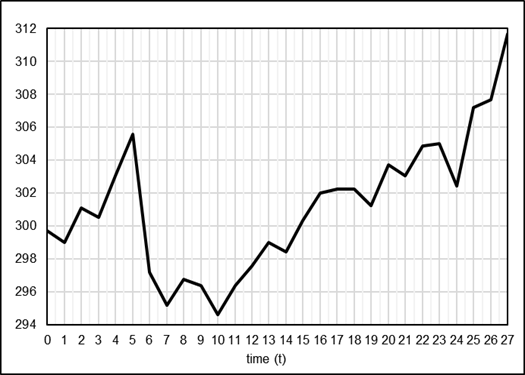
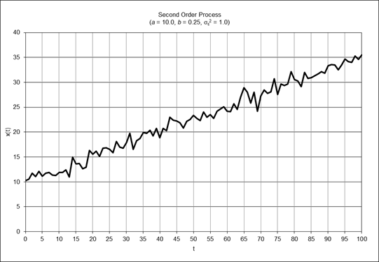
The following graph shows an example of a time series based on an underlying second order process:

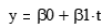
A time series regression model based on a second order process has the form:

where y is the dependent variable, β₀ is the estimated mean, and β₁ is the estimated linear trend. The model parameter β₀ corresponds to the coefficients of a second order process mean filter, and the model parameter β₁ corresponds to the coefficients of a second order process linear trend filter.

Note that this type of regression model is commonly referred to as “linear regression”, which assumes a linear relationship between the dependent and independent variables.

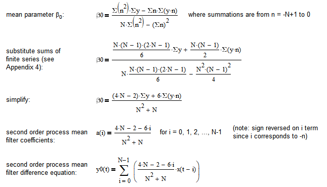
Second Order Process Mean Filter

Appendix 2a shows the derivation of the difference equation of the second order process mean filter, which is:

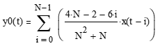
The second order process mean filter is a type of FIR low pass filter. The value N (N > 2) determines the -3 dB cutoff frequency, which is inversely proportional to N (the cutoff period P_c is proportional to N).

This filter is sometimes also called an “end point moving average” or a “least squares moving average”.

Second Order Process Mean Filter Frequency Response (N = 10)

Example: Second order process mean filter with length N = 10

Passes frequencies below the -3 dB cutoff frequency f_c of approximately 0.11, which corresponds to a cutoff period P_c of approximately 9.091 time samples. There is a magnitude peak above 1.0 (i.e., 0 dB) at a period of approximately 18 time samples.

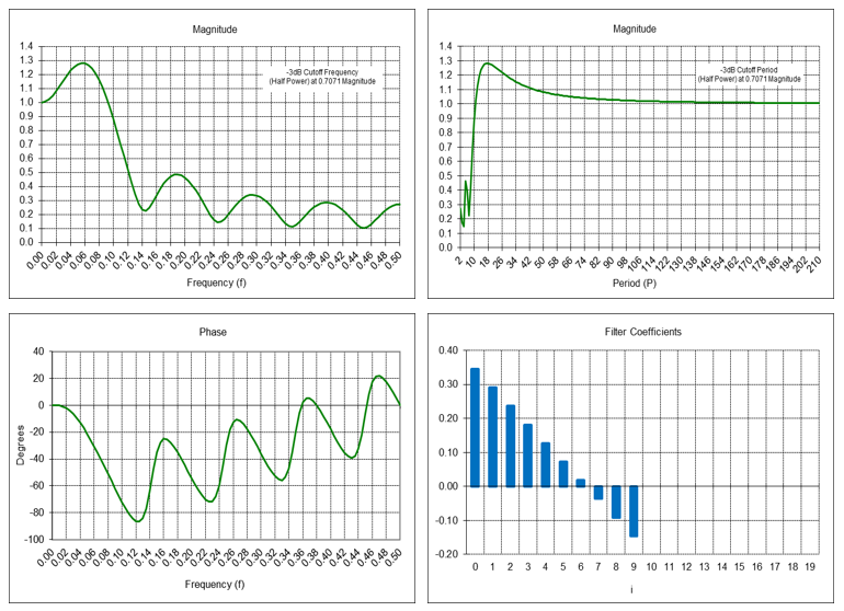
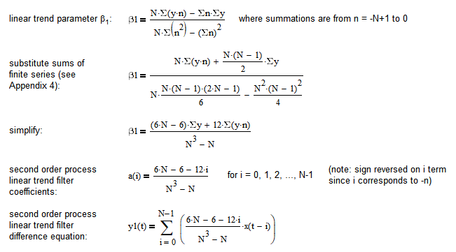
Second Order Process Linear Trend Filter

Appendix 2b shows the derivation of the difference equation of the second order process linear trend filter, which is:

The second order process linear trend filter is a type of FIR bandpass filter. A bandpass filter passes frequencies between a low -3 dB cutoff frequency f_L and a high -3 dB cutoff frequency f_H, called the bandwidth (Δf = f_H – f_L), and attenuates the others. The filter has a center (also called “resonant”) frequency f₀, which the filter passes at maximum power. The value N (N > 2) determines the center frequency, which is inversely proportional to N (the center period P₀ is proportional to N).

This filter is the same as the Linear Regression Slope indicator.

Second Order Process Linear Trend Filter Frequency Response (N = 10)

Example: Second order process linear trend filter with length N = 10

The center frequency f₀ is approximately 0.065, which corresponds to a center period P₀ of approximately 15.38 time samples.

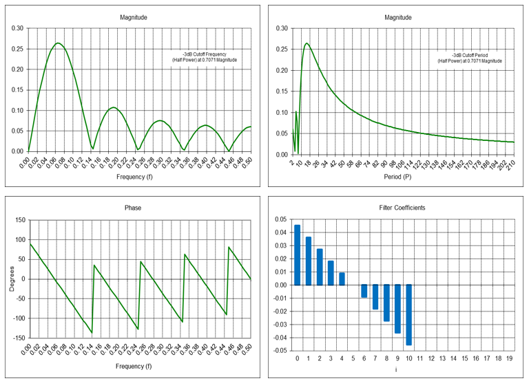
Second Order Process Mean and Linear Trend Filter Example

The chart below shows the second order process mean filter (green dashed line) and second order process linear trend filter (blue line), both with filter lengths N = 10, applied to the daily S&P 500 index for the year 2023.

The amplitude of the second order process linear trend filter output is proportional to the local slope of the price, i.e., the greater the amplitude, the steeper the slope, although the output can be affected by the presence of cycles and non-linear trends.

Trading Signal Generation

Trading signals using second order process mean and linear trend filters can potentially be generated, for example, when:

• the price crosses above (buy) or below (sell) the mean line,
• the mean line reaches a local crest (sell) or trough (buy),
• the linear trend line crosses above (buy) or below (sell) the zero line,
• the linear trend line reaches a local crest (sell) or trough (buy),

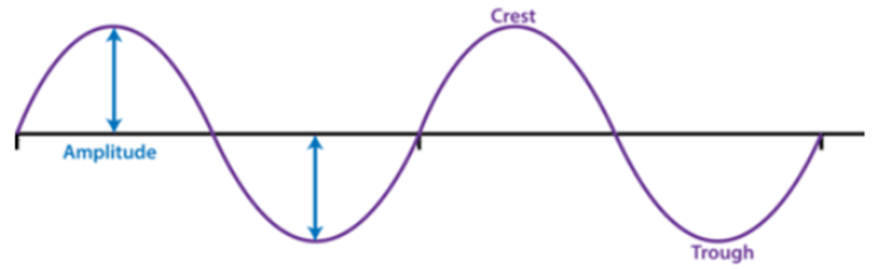
or by a combination of these conditions. Some of these trading signals are indicated by the lines at the bottom of the chart. The graph below illustrates the concepts of amplitude, crest, and trough:

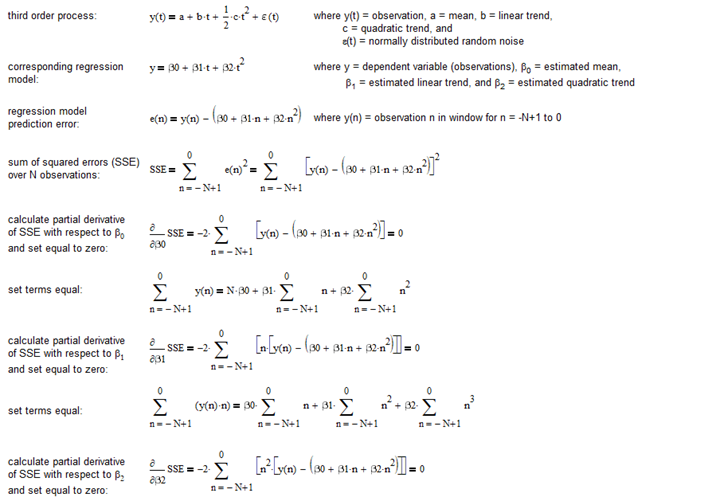
6. Third Order Process Filters

A time series based on a third order process consists of a mean a, a linear trend b, and a quadratic trend c which is contaminated with random normally distributed noise ε(t) where ε(t) ~ N(0, σ_ε²):

y(t) = a + b*t + ½*c*t² + ε(t)

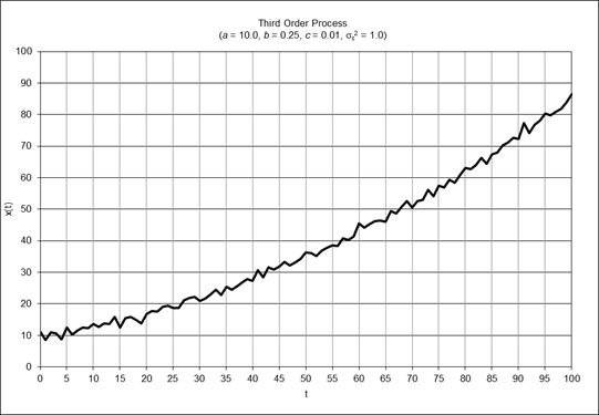
The following graph shows an example of a time series based on an underlying third order process:

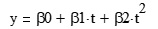
A time series regression model based on a third order process has the form:

where y is the dependent variable, β₀ is the estimated mean, β₁ is the estimated linear trend, and β₂ is the estimated quadratic trend. The model parameter β₀ corresponds to the coefficients of a third order process mean filter, the model parameter β₁ corresponds to the coefficients of a third order process linear trend filter, and the model parameter β₂ corresponds to the coefficients of a third order process quadratic trend filter.

Note that this type of regression model is commonly referred to as “polynomial regression”, where the relationship between the dependent variable and the independent variables is modeled using a non-linear expression such as a quadratic, cubic, or higher order equation.

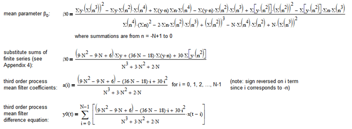
Third Order Process Mean Filter

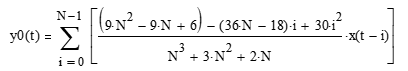
Appendix 3a shows the derivation of the difference equation of the third order process mean filter, which is:

The third order process mean filter is a type of FIR low pass filter. The value N (N > 3) determines the -3 dB cutoff frequency, which is inversely proportional to N (the cutoff period P_c is proportional to N).

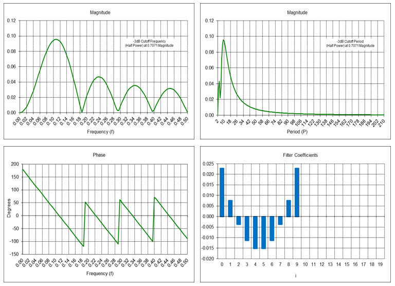
Third Order Process Mean Filter Frequency Response (N = 10)

Example: Third order process mean filter with length N = 10

Passes frequencies below the -3 dB cutoff frequency f_c of approximately 0.165, which corresponds to a cutoff period P_c of approximately 6.061 time samples. There is a magnitude peak above 1.0 (i.e., 0 dB) at a period of approximately 10 time samples.

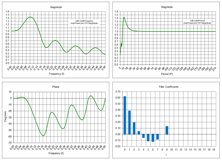
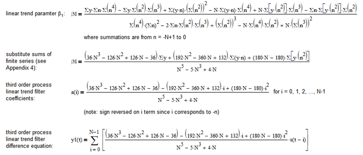
Third Order Process Linear Trend Filter

Appendix 3b shows the derivation of the difference equation of the third order process linear trend filter, which is:

The third order process linear trend filter is a type of FIR bandpass filter. The filter has a center frequency f₀, corresponding to a center period P₀, which passes at maximum power. The value N (N > 3) determines the center frequency f₀, which is inversely proportional to N (the center period P₀ is proportional to N).

Third Order Process Linear Trend Filter Frequency Response (N = 10)

Example: Third order process linear trend filter with length N = 10

The center frequency f₀ is approximately 0.105, which corresponds to a center period P₀ of approximately 9.52 time samples.

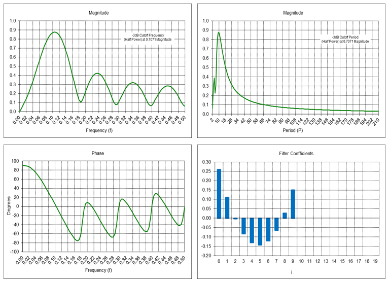
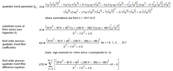
Third Order Process Quadratic Trend Filter

Appendix 3c shows the derivation of the difference equation of the third order process quadratic trend filter, which is:

The third order process quadratic trend filter is a type of FIR bandpass filter. The filter has a center frequency f₀, corresponding to a center period P₀, which passes at maximum power. The value N (N > 3) determines the center frequency f₀, which is inversely proportional to N (the center period P₀ is proportional to N).

Third Order Process Quadratic Trend Filter Frequency Response (N = 10)

Example: Third order process quadratic trend filter with length N = 10

The center frequency f₀ is approximately 0.11, which corresponds to a center period P₀ of approximately 9.091 time samples.

Third Order Process Mean, Linear Trend, and Quadratic Trend Filter Example

The chart below shows the third order process mean filter (green dashed line), the third order process linear trend filter (blue line), and the third order process quadratic trend filter (red line), all with filter lengths N = 10, applied to the daily S&P 500 index for the year 2023.

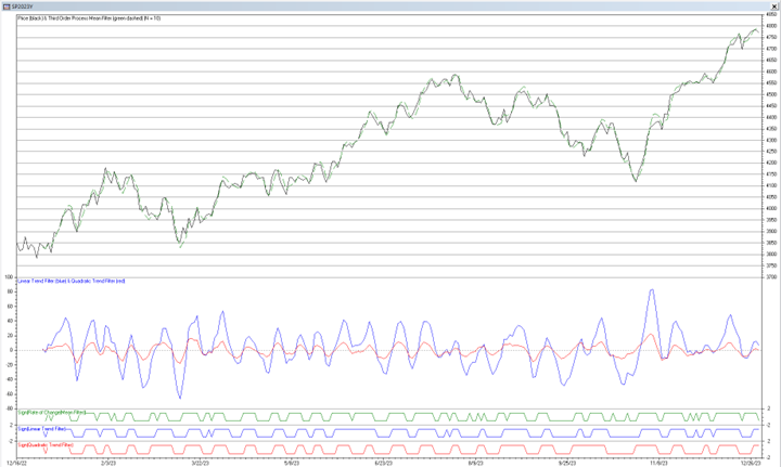
The amplitude of the third order process linear trend filter output is proportional to the local slope of the price, i.e., the greater the amplitude, the steeper the slope. Similarly, the amplitude of the third order process quadratic trend filter output is proportional to the local slope of the linear trend. However, the output of both of these latter two filters can be affected by the presence of cycles and higher order trends.

Trading Signal Generation

Trading signals using third order process mean, linear trend, and quadratic trend filters can potentially be generated, for example, when:

• the price crosses above (buy) or below (sell) the mean line,
• the mean line reaches a local crest (sell) or trough (buy),
• the linear trend line crosses above (buy) or below (sell) the zero line,
• the linear trend line reaches a local crest (sell) or trough (buy),
• the quadratic trend line crosses above (buy) or below (sell) the zero line,
• the quadratic trend line reaches a local crest (sell) or trough (buy),

or by a combination of these conditions. Some of these trading signals are indicated by the lines at the bottom of the chart.

7. Comments

Relation to Savitzky-Golay Filters

The filters analyzed in this article are related to Savitzky-Golay filters [6]. Savitzky-Golay filters were originally developed to smooth noisy data obtained from chemical spectrum analyzers. There are two types: smoothers and differentiators. As with the filters discussed in this article, the design of Savitzky-Golay filters is also based on a least squares fit of the observations to a polynomial function, where the degree of the polynomial is selected based on the structure of the observations.

Savitzky-Golay smoothers are technically not filters per se. The terms “smoothing” and “filtering” are often used interchangeably but are actually somewhat different:

• smoothing – uses past and current observations to estimate previous states
• filtering – uses past and current observations to estimate the current state
• prediction – uses past and current observations to forecast future states.

The output of differentiators is proportional to the rate of change (i.e., the derivative with respect to time) of the input. As with the filters derived in this article, the frequency responses of Savitzky-Golay differentiators resemble those of FIR bandpass filters, which act as differentiators over a certain range of their frequency response, i.e., between f = 0 and (roughly) the center frequency f₀.

The outputs of Savitzky-Golay smoothers and differentiators are traditionally taken at the center or midpoint of the observation window, so an odd number of observations is normally used. In contrast, the output of the filters analyzed in this article is taken at the most recent observation window end point and can use an odd or even number of observations. As an example, the commonly-used moving average is a filtering operation where the output is taken at the end point of the observations, whereas a centered moving average is a smoothing operation where the output is taken at the center point. The difference between the two is illustrated by the following charts:

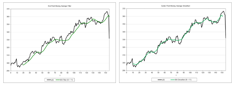
Filter outputs that are coincident with the most recent observations are generally more useful to technical analysts and traders.

Other Types of Filters Based on Time Series Process Models

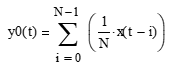
Previous articles in this series have examined other types of digital filters that are also modeled on the same three time series process assumptions:

• “An Introduction to Digital Signal Processing for Trend Following” – filters modeled on first order processes, specifically moving averages, linear weighted moving averages, exponential smoothing, and time series momentum [5].
• “Trend-Following Filters – Part 1/2” – filters modeled on second order processes, specifically double moving averages, double linear weighted moving averages, double exponential smoothing, and alpha-beta tracking filters [7].
• “Trend-Following Filters – Part 2/2” – filters modeled on third order processes, specifically triple moving averages, triple linear weighted moving averages, triple exponential smoothing, and alpha-beta-gamma tracking filters [8].

Acknowledgements

I would like to thank Valeriy Zakamulin for reviewing this article and providing several helpful comments and suggestions.

Appendix 1 – First Order Process Filter Derivation

Appendix 2 – Second Order Process Filter Derivations

a. Mean Filter Coefficients Derivation from Parameter β₀

b. Linear Trend Filter Coefficients Derivation from Parameter β₁

Appendix 3 – Third Order Process Filter Derivations

a. Mean Filter Coefficients Derivation from Parameter β₀

b. Linear Trend Filter Coefficients Derivation from Parameter β₁

c. Quadratic Trend Filter Coefficients Derivation from Parameter β₂

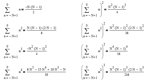
Appendix 4 – Sums of Finite Series

References

[1] Spurr, W. A. & Bonini, C. P., Statistical Analysis for Business Decisions, Richard D. Irwin, 1967.

[2] STAT 501, Eberly College of Science, Pennsylvania State University, 2024; available online at https://online.stat.psu.edu/stat501/.

[3] “Linear Regression Slope Indicator: Market Trends with Precision”, 2024, available online at https://tradingliteracy.com/linear-regression-slope-indicator/.

[4] “What is TSF? Understanding Time Series Forecast Indicator”, 2022, available online at https://quantstrategy.io/blog/what-is-tsf-understanding-time-series-forecast-indicator/.

[5] Stern, H., “An Introduction to Digital Signal Processing for Trend Following”, August 2020, updated September 2023; available online at https://alphaarchitect.com/2020/08/an-introduction-to-digital-signal-processing-for-trend-following/.

[6] Savitzky, A. & Golay, M. J. E., “Smoothing and Differentiation of Data by Simplified Least Squares Procedures”, Analytical Chemistry, 36 (8), 1627-1639, July 1964; available online at http://constans.pbworks.com/w/file/fetch/121217343/SavitskyGolay.pdf.

[7] Stern, H., “Trend-Following Filters – Part 1/2” December 2020; available online at https://alphaarchitect.com/2020/12/29/trend-following-filters-part-1-2/.

[8] Stern, H., “Trend-Following Filters – Part 2/2”, January 2021;  available online at https://alphaarchitect.com/2021/01/21/trend-following-filters-part-2-2/.