Trend-Following Filters – Part 3

Introduction

This is the third article in a series of three, the first two are available here and here. Those articles focus on examining from a digital signal processing (DSP) perspective⁽¹⁾ various types of digital filters that are designed to model trends in time series, in order to illustrate their properties and limitations. This article discusses a different signal processing tool called a “filter bank”.

Filter banks are used in many areas of electrical engineering, telecommunications, and other fields in applications such as audio, video, and image noise reduction, compression, storage, and transmission. A familiar example of a filter bank is the audio graphic equalizer, which can be used to alter music sound quality, e.g., to boost bass frequencies, which are generally between 20 and 300 Hertz (cycles per second), relative to treble frequencies, which are generally between 2,000 and 16,000 Hertz.

1. Digital Analysis-Synthesis Filter Bank

Filter banks⁽²⁾ can be designed to work with either continuous-time analog signals, such as music and speech, or discrete-time digital signals, such as high-definition television and wireless communication. The general form of a digital filter bank that can be used to implement a range of different operations is called an “M-band digital analysis-synthesis filter bank” and is comprised of three parts:

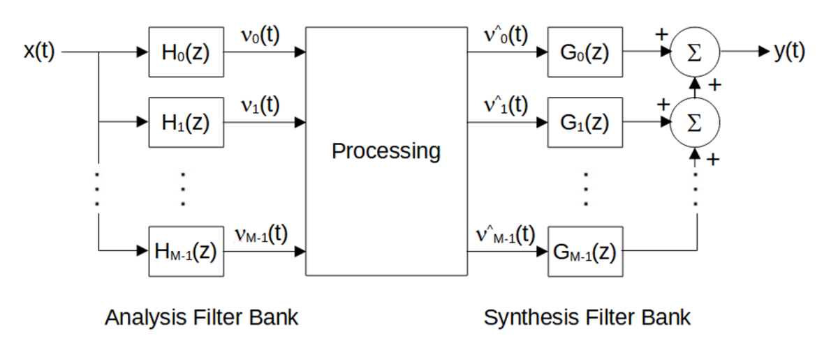
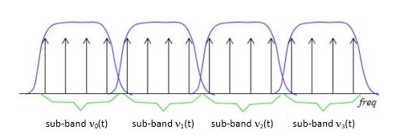
• Analysis filter bank – Splits the input signal x(t) at each integer time step t into an M number of frequency components (M > 1), called “sub-bands”, using a set of digital filters arranged in parallel. Each filter in the analysis filter bank is designed to pass a specific frequency sub-band ν_i(t), with each sub-band occupying a portion of the original frequency band of x(t). These filters are represented by the H_i(z) blocks in the diagram above.

• Processing – Performs transformations, such as compression, on the individual sub-bands, based on the filter bank design objective. The processed sub-band outputs are represented by ν^_i(t).
• Synthesis filter bank – Combines the processed sub-band outputs into a single output signal y(t) using addition. The synthesis operation can include ancillary filtering operations, represented by the G_i(z) blocks.

2. Example Digital Analysis-Synthesis Filter Bank

The following example illustrates the digital analysis-synthesis filter bank concept. The design objective is to produce a “de-noised” output y(t) of the input time series x(t).

The three parts of the example filter bank are as follows:

• Analysis filter bank – The analysis filter bank is comprised of a set of six second-order IIR bandpass digital filters (M = 6). The details of the bandpass filter design are described in the Appendix. The center periods P₀ of the six filters are set to 15, 88, 513, 2990, 17427, and 101572 time samples, respectively, in order to have nonoverlapping passbands at the -3 dB (half-power) period cutoff points of the filters. This arrangement effectively attenuates short periods below around 6 time samples, which are considered to be “noise” with respect to daily data (i.e., an input x(t) sampling interval of once per trading day at the market close) for the purposes of the example, while passing the longer periods. The quality factor Q of each filter is set to 0.5, i.e., critically damped (see the Appendix), in order to balance filter output responsiveness versus lag.
• Processing – No additional processing is performed. The analysis filter bank outputs ν_i(t) are passed directly to the synthesis filter bank inputs ν^_i(t).
• Synthesis filter bank – The G_i(z) filters adjust the gain of each ν^_i(t) using multiplication so that the average maximum passband magnitude of the output y(t) is approximately 1.0 (0 dB):

G_i(z) = 0.886

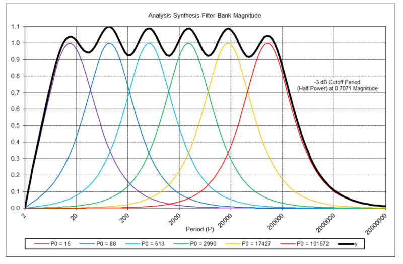
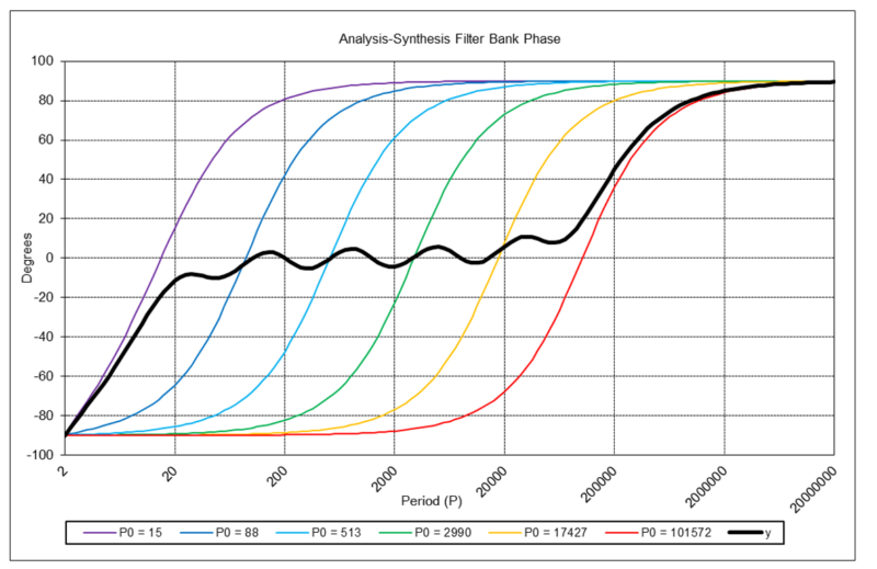
The graphs below show the magnitude and phase spectrums of the individual analysis filter bank outputs ν_i(t) and the synthesis filter bank output y(t). Note that the horizontal x-axis of both graphs uses a base-10 logarithmic scale, which is nonlinear.

3. Example Filter Bank Applications

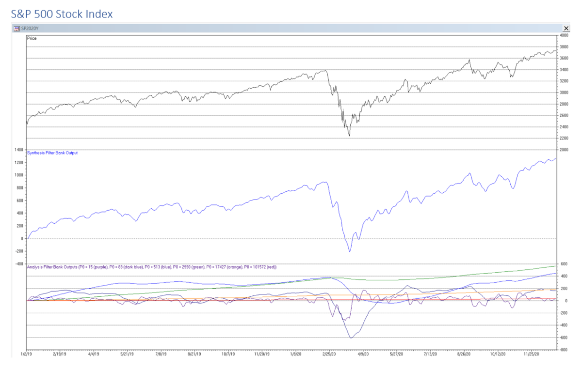
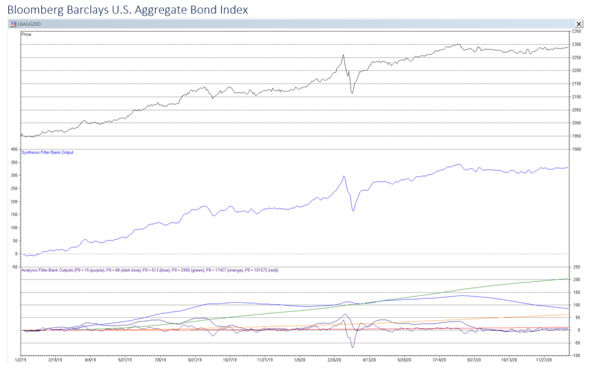
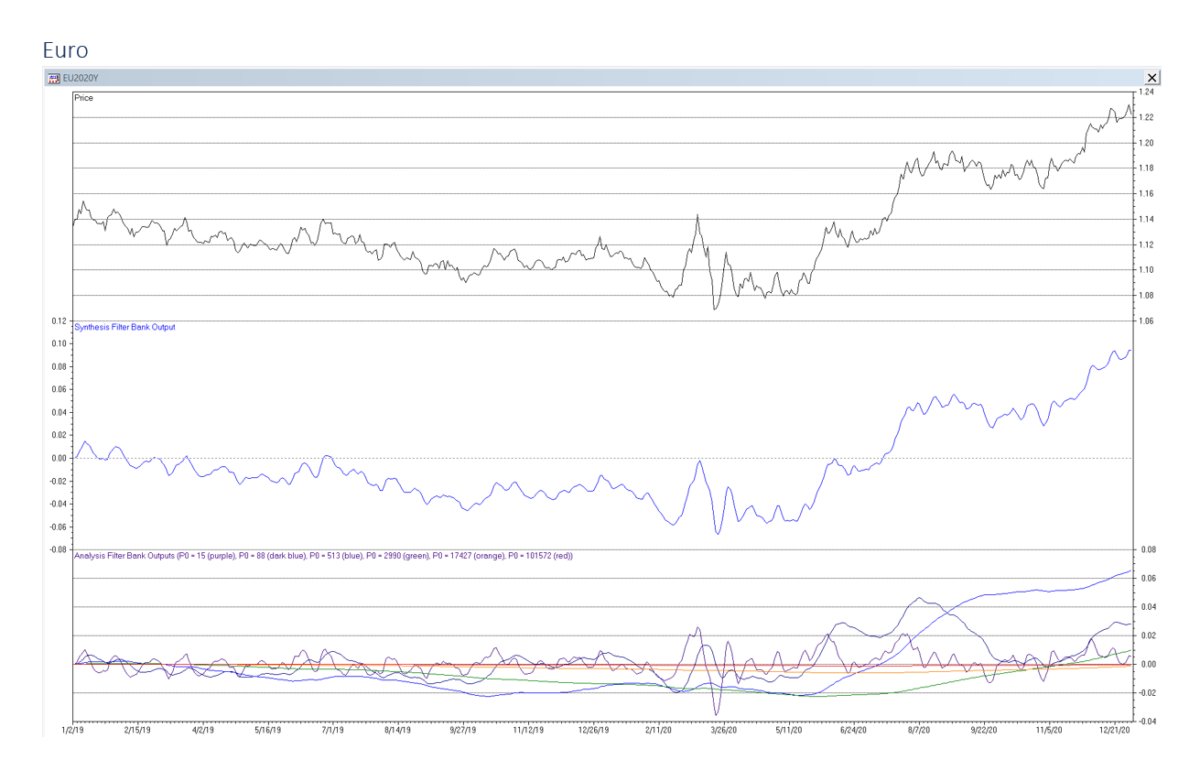
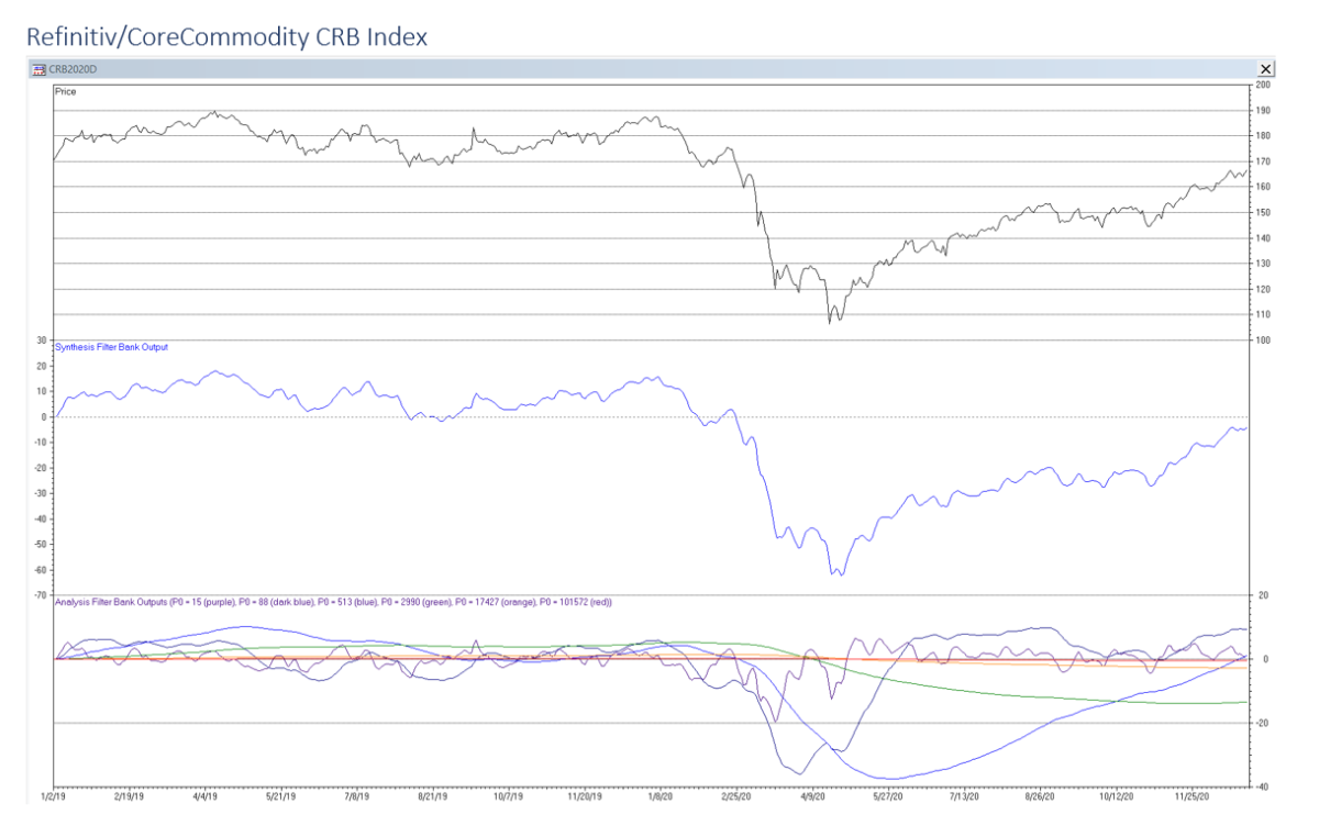
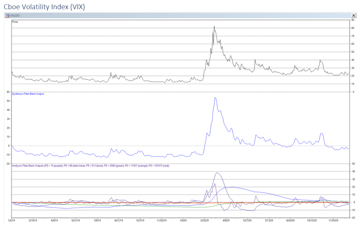
The following charts show the result of applying the example digital analysis-synthesis filter bank to the daily closing values of a stock index, a bond index, a currency, a commodity index, and a volatility index for the years 2019 and 2020. The input index or price time series x(t) is shown in the top section of each chart, the synthesis filter bank output y(t) is shown in the middle section, and the individual analysis filter bank outputs ν_i(t) are shown in the bottom section.

Note that the analysis filter bank outputs and the synthesis filter bank output fluctuate around the zero line, since the analysis bandpass filters remove the zero frequency (f = 0) component of the input x(t). This component can be thought of as the steady direct current (DC) level of the input over the time period.

4. Trading Signal Generation

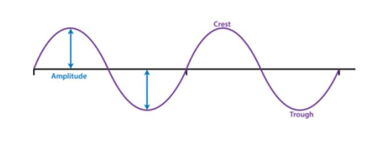
Trading signals can potentially be generated, for example, when the filter bank output y(t) reaches a local trough (buy) or crest (sell), since, as explained in the next section, it is closely coincident with the start and end of trends as well as the bottoms and tops of cycles in the input x(t).

The individual analysis filter outputs ν_i(t) can be used to evaluate the relative amplitude (strength) of the associated frequency sub-band components.

5. General Comments on Filter Banks

The example analysis-synthesis filter bank magnitude spectrum graph shows the magnitude response of the individual analysis bandpass filter outputs ν_i(t) and the synthesis filter bank output y(t). In particular, the magnitude spectrum of y(t) is relatively flat, with a small amount of oscillation, from approximately 10 to 160,000 time samples, indicating little amplitude distortion over that range.

The example analysis-synthesis filter bank phase spectrum graph shows the phase angles of the individual analysis bandpass filter outputs ν_i(t) and the synthesis filter bank output y(t). Generally speaking, “phase” measures the relative time difference between two sine waves but expressed relative to the sine wave period instead of in time units, specifically as an angle in either degrees or radians. For example, a phase angle of 90 degrees is a shift of ¼ of the complete one-period sine wave cycle of 360 degrees. A negative phase angle indicates lag (i.e., time delay) and a positive angle indicates lead. In the case of the example filter bank output y(t), the phase angle oscillates around zero degrees from approximately 15 to 100,000 time samples, indicating it is close to having a true “zero lag” over this range. However, there is phase lag between the Nyquist period of 2 and 15 time samples and phase lead above approximately 100,000 time samples. The lag is associated with the noise attenuation of the filter bank, since there is an inherent trade-off between noise reduction and lag. The lead is associated with the bandpass filter having the longest center period P₀ = 101572.

The use of multiple filters in a filter bank that operate on separate frequency components avoids many of the limitations of using a single fixed-coefficient filter with non-stationary financial time series. This applies to:

• lowpass filters, such as moving average (MA), linear weighted moving average (LWMA), and exponential smoothing (ES), which typically suffer from significant lag,
• differentiator filters, such as time-series momentum (TSMOM), which can have poor noise suppression, and
• bandpass filters, such as moving average crossover (MAC) and moving average convergence-divergence (MACD), which are only able to be tuned to specific center frequencies and have associated bandwidth limits.

Filter banks can also serve as an alternative to adaptive filtering. A digital adaptive filter employs time-varying coefficients, which are adjusted dynamically using an optimization algorithm, to minimize the error between the filter output and the desired signal. However, adaptive filtering algorithms can often be complex to implement and do not always respond rapidly enough to the volatility and non-stationarity of financial time series to be useful for trading purposes.

Finally, the example filter bank is just one of many different possible designs. It is intended for illustrative purposes only and should not be considered to be “suggested” or “optimal”. Several different elements can be modified to potentially improve the response and other characteristics of a filter bank, for example:

• the type of bandpass filter, e.g., infinite impulse response (IIR) versus finite impulse response (FIR)
• the number M of bandpass filters in the analysis filter bank
• the analysis bandpass filter center periods P₀, quality factor Q values, and associated cutoff periods P_S and P_L (see the Appendix).

Note that rapid reversals in price trends are usually difficult to distinguish in real-time from noise and short-term volatility, in particular, because they all fall into the same general short period (high frequency) range. As a result, the noise cutoff period of the filter bank needs to be carefully chosen, for example, with respect to the input x(t) sampling interval (hourly, daily, weekly, monthly, etc.), to produce an acceptable balance between responsiveness to the start and end of trends, which can often be abrupt, on one hand, and susceptibility to noise and short-term volatility, which can result in loss-making “whipsaw” trades, on the other. The larger the noise cutoff period, the greater the lag in the short period range.

Acknowledgements

I would like to thank Larry Stabile for reviewing this article and providing many helpful comments and suggestions.

References

1. Diniz, P. S. R., da Silva, E. A., B., and Netto, S. L., Digital Signal Processing – System Analysis and Design, Cambridge University Press, 2010.
2. Oppenheim, A. V. and Schafer, R. W., Discrete-Time Signal Processing, Prentice Hall, 1989.
3. Orfanidis, S. J., Introduction to Signal Processing, Prentice-Hall, 1996.
4. Lane, J. and Hillman, G., Implementing IIR/FIR Filters with Motorola’s DSP56000/DSP56001, APR7/D, Rev 1, Motorola, Inc., 1991.

Appendix – Second-Order IIR Bandpass Filter

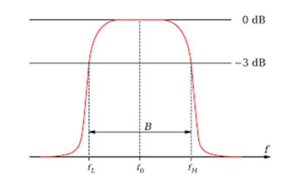
A bandpass filter passes frequencies between the -3 dB (half-power) low cutoff frequency f_L (corresponding to long cutoff period P_L = 1/f_L) and the high cutoff frequency f_H (corresponding to short cutoff period P_S = 1/f_H). In particular, a bandpass filter has a center (also called “resonant”) frequency f₀ (corresponding to center period P₀ = 1/f₀), which is passed at maximum power (0 dB). The frequency range between f_L and f_H is called the “passband”. The filter attenuates frequencies above and below the passband. The difference between f_L and f_H is called the “bandwidth” of the filter, denoted by B in the diagram below. Various bandpass filter designs are available, including for both finite impulse response (FIR) and infinite impulse response (IIR) filter types.

A more thorough treatment of bandpass filters can be found in a number of texts, in particular: 2. Discrete-Time Signal Processing and 3. Introduction to Signal Processing.

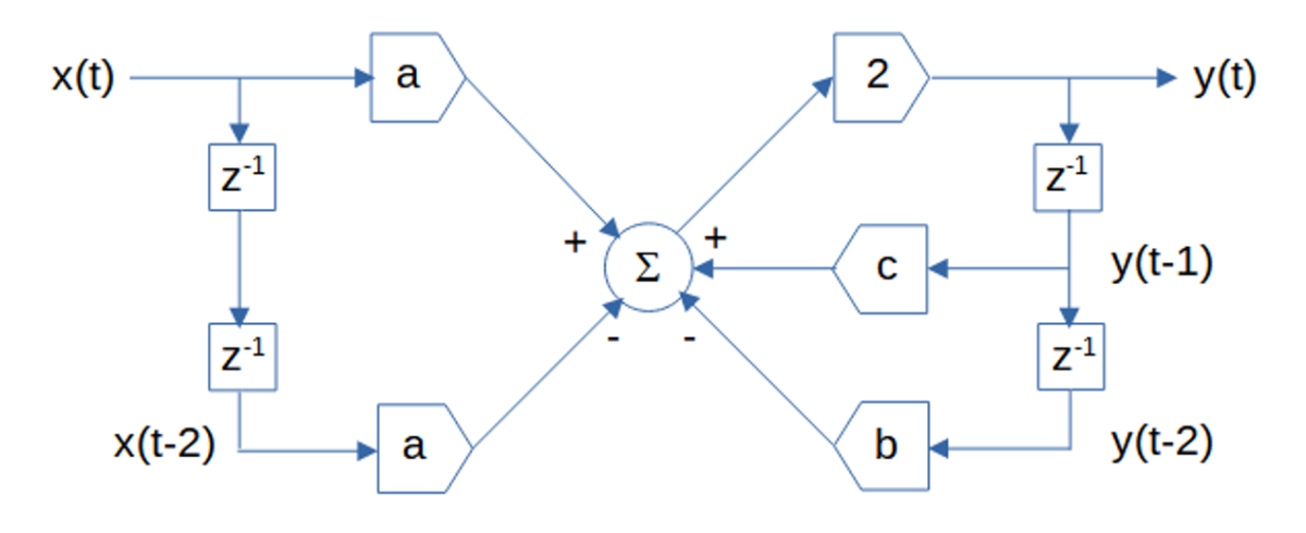
The filter used in the analysis filter bank example is a particular type of second-order IIR bandpass filter, which is described in detail in 4. G., Implementing IIR/FIR Filters with Motorola’s DSP56000/DSP56001. The filter implements the following IIR difference equation.

where:

• P₀ = center period (number of time samples to complete one cycle)
• f₀ = center frequency (number of cycles per time sample) = 1/P₀
• B = frequency bandwidth = f_H – f_L
• Q = quality factor = f₀/B
• b = ½*[1 – tan((2*π*f₀)/(2*Q))] / [1 + tan((2*π*f₀)/(2*Q))]
• c = (½ + b)*cos(2*π*f₀)
• a = ½*(½ – b)

The quality factor Q controls the bandwidth B of the filter relative to its center frequency f₀. In general, a small quality factor Q value results in a wide bandwidth, and a large quality factor Q value results in a narrow bandwidth. Values of Q fall into three qualitative ranges:

• overdamped (0 < Q < 0.5) – The output response to a unit pulse input decays exponentially to a steady-state value with no oscillation. The smaller the value of Q, the slower the rate of decay.
• critically damped (Q = 0.5) – The output response to a unit pulse input returns to a steady-state value in the shortest time and with no oscillation.
• underdamped (Q > 0.5) – The output response to a unit pulse input decays exponentially to a steady-state value with oscillation. The greater the value of Q, the slower the rate of decay and the longer the oscillation persists.

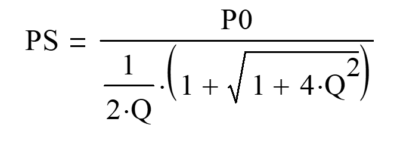
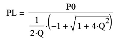
The bandpass filter -3 dB (half-power) cutoff periods can be calculated from the center period P₀ and quality factor Q as follows:

• -3 dB short cutoff period P_S:

• -3 dB long cutoff period P_L: