Trend-Following Filters – Part 6

1.    Introduction

This article analyzes six trend-following indicators from a digital signal processing (DSP) frequency domain perspective in which the indicators are considered as digital filters and their frequency response characteristics are determined. In addition, potential trading signals generated by each indicator in the time domain are displayed graphically by applying the indicator to the monthly S&P 500 index for the years 1990 to 2022.

The six indicators are:

• 10-month price minus moving average – commonly used with tactical asset allocation models that shift allocations in a portfolio across a set of asset classes on a monthly basis
• 12-month time series momentum – often used as an alternative to the 10-month price minus moving average indicator
• moving average crossover – a popular market timing indicator originally designed for use with daily prices and modified here for use with monthly prices in an example
• moving average convergence-divergence – an alternative to the moving average crossover indicator, also originally designed for use with daily prices and modified here for use with monthly prices in an example
• Markov Switching Model rule – a trend-following rule based on a stock market state model, which was recently published in an academic paper
• Semi-Markov Switching Model NB(4) rule – a trend-following rule based on a more complex stock market state model, also published in the same paper.

Frequency domain analysis can often offer unique insights into the general behavior of an indicator, as opposed to being limited to examining it in specific scenarios in the time domain.

2.    Basic DSP Concepts

This section provides an overview of the DSP concepts mentioned in this article. Detailed discussions of these topics can be found in various text books and lecture notes, such as [1]. Additional discussion of DSP concepts, as well as of several of the indicators from a DSP perspective, can be found in [2].

Time Domain and Frequency Domain

Financial time series that are structured as data sampled at a uniform time interval, e.g., hourly, daily, weekly, or monthly, are called discrete-time time series and referred to as being in the “time domain”. A graph in the time domain, such as a price chart, displays the time series value at each time sample. Technical analysts generally study price data in the time domain, and the output of most technical analysis indicators is also usually calculated and displayed in the time domain.

The Fourier theorem states that a general function, however complicated, may be expressed as the sum of sinusoidal functions or frequency components, each of which has a specific amplitude (a measure of maximum displacement from equilibrium) and phase (a measure of angular offset). While Fourier analysis was originally developed for continuous-time functions, such as analog signals, it is also applicable in a modified form to discrete-time functions. Digital signals and discrete-time time series represented in this way are referred to as being in the “frequency domain”.

Frequency and Period

For digital signals and discrete-time time series containing cycles, i.e., sinusoidal-like patterns, two related measurements, frequency and period, can be used. Frequency (f) is the number of cycles completed per time sample of the signal or time series, whereas period (P) is the cycle length, i.e., the number of time samples to complete one cycle. Period is the reciprocal of frequency, where P = 1/f. Frequency can also be stated as the number of radians (ω) per time sample where 2*π radians = 360 degrees and ω = 2*π*f. In this article, period is used as the measurement, since it is commonly utilized by and most familiar to technical market analysts studying financial time series.

Types of Filters

Digital filtering is widely used in electrical engineering, telecommunications, and other fields to process digital signals, e.g., to alter the features of the input signal in a particular way, which appears in the filter output. Digital filters are categorized and viewed in terms of their effect on the frequencies of the signal passing through them. There are four basic types of filters:

• low pass – passes low frequencies (long periods) and attenuates high frequencies (short periods)
• high pass – passes high frequencies (short periods) and attenuates low frequencies (long periods)
• bandpass – passes frequencies (periods) within a specific range or bandwidth and attenuates the others
• bandstop – attenuates frequencies (periods) within a specific range or bandwidth and passes the others.

Another type of filter is a differentiator, where the filter output is proportional to the rate of change, i.e., the derivative with respect to time, of the input.

Finite Impulse Response Filter

A finite impulse response (FIR) filter uses only current and past input values in its calculation, i.e., it does not use feedback and hence is non-recursive. As a result, the filter response in the time domain to a unit pulse input is finite (see Section 2 of [2] for additional details). The general equation of a FIR filter is:

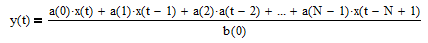
where

• N = number of filter input samples
• x(t-i) = filter input sample at integer time t-i for i = 0, 1, 2, …, N-1
• a(i) = filter coefficient of filter input x(t-i)
• y(t) = filter output at integer time t
• b(0) = filter coefficient of filter output y(t).

Infinite Impulse Response Filter

An infinite impulse response (IIR) filter uses current and past input values as well as past output values in its calculation, i.e., it uses feedback and hence is recursive. As a result, the filter response in the time domain to a unit pulse input is infinite (see Section 2 of [2] for additional details). The general equation of an IIR filter is:

where

• N = number of filter input samples
• M = number of filter output samples
• x(t-i) = filter input sample at integer time t-i for i = 0, 1, 2, …, N-1
• a(i) = filter coefficient of filter input x(t-i)
• y(t-i) = filter output sample at integer time t-i for i = 0, 1, 2, …, M-1
• b(i) = filter coefficient of filter output y(t-i).

Frequency Response

All six of the indicators discussed in this article act as digital linear time-invariant (LTI) filters and are completely characterized by their response in the frequency domain. There are two components of frequency response:

• magnitude response – the ratio of the amplitude of the filter output to the amplitude of the filter input across a range of frequencies or periods
• phase response – the angular shift, i.e., time delay, of the filter output relative to the filter input, measured in radians or degrees, across a range of frequencies or periods.

See Appendix 1 for the calculation of frequency response.

Cutoff Frequency or Period

One gauge of filter frequency response is the cutoff frequency or period, which is the frequency or period at which the power of the filter output is reduced by a certain amount relative to the power of the input. Signal power is the square of signal amplitude. A standard cutoff frequency or period benchmark used in filter design and analysis is the frequency or period at which the power of the filter output is one-half the power of the filter input, which corresponds to a reduction of -3 decibels (-3 dB). (See Section 2 of [2] for calculation details.)

3.    Spectral Analysis of the Monthly S&P 500 Stock Index 1990-2022

The monthly S&P 500 stock index closing values from 1990 to 2022, which include 396 months (33 years) of time samples, are used in this article to illustrate the trading signals that can potentially be generated by the indicators in the time domain. This section illustrates this time series in both the time and frequency domains.

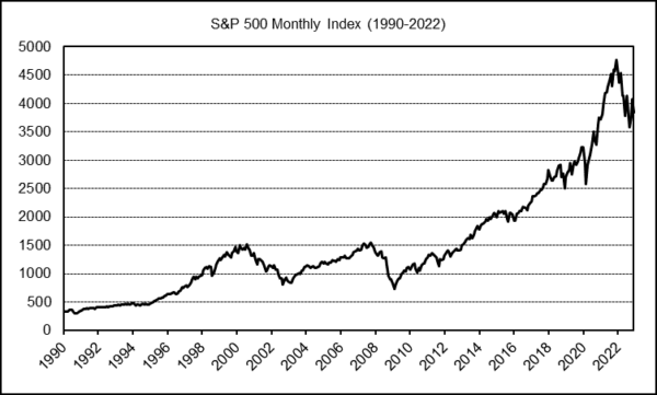
Time Domain Representation

A chart of the monthly 1990 to 2022 S&P 500 index closing values is shown below. The time series is marked by the dot-com bubble of the late 1990’s, the dot-com bust starting in 2000, the recovery starting in 2003, the Great Recession of 2008, the recovery from 2009 to 2019, the pandemic dip in early 2020 and subsequent bull market, and, finally, the 2022 correction. The index values range from the October 1990 low of 304.00 to the December 2021 high of 4766.18.

Frequency Domain Representation

Discrete-time signals and time series can be converted from the time domain to the frequency domain using the Discrete Fourier Transform (DFT). The output of the DFT is the frequency spectrum of the signal or time series. Details concerning spectral analysis and the DFT can be found in various textbooks and lecture notes, such as [1] and [3]. See Appendix 2 for the calculation of the DFT.

There are two components of the frequency spectrum:

• amplitude – the amplitude of each frequency or period component across a range of frequencies or periods
• phase – the angular shift of each frequency or period component across a range of frequencies or periods, measured in radians or degrees.

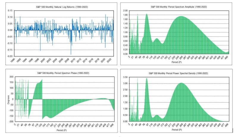
Below in the upper left is a graph of the S&P 500 index natural log (i.e., continuously compounded) monthly returns for 1990 to 2022. The natural log monthly returns are used in the DFT to calculate the frequency spectrum. The log returns range from the October 2008 minimum of -0.1856 to the April 2020 maximum of 0.1194, with a mean of 0.0060. The standard deviation is 0.0434, the skewness is -0.7257, and the kurtosis is 1.3979.

Below in the upper right is a graph of the spectrum amplitude of the log returns, displayed in terms of period. Below lower left is a graph of the spectrum phase in degrees, also displayed in terms of period (see the note regarding “phase wrap” in Section 5 of [2]). Finally, below lower right is a graph of the power spectral density (PSD) of the period spectrum amplitude. The PSD calculates the power present in the signal or time series as a function of frequency or period, where power is calculated as the square of the amplitude. The graph shows power peaks at periods of approximately 4, 6, 24, 43, 88, and 262 months. Very short periods (high frequencies) are generally associated with “noise”. As noted in [8], a study found that, as measured using the S&P 500 index over the years 1835 to 1997, the average duration of a bull market is approximately 29 months and the average duration of a bear market is approximately 15 months, adding up to an average market cycle length of 44 months, which happens to closely coincide with the 43 month peak observed in the PSD graph.

4.    10-Month Price Minus Moving Average

The 10-month moving average (MA) indicator was researched and popularized by Meb Faber [4]. A MA filter is a FIR low pass filter. The equation of a MA filter with a length of N integer time samples is:

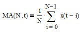
The MA filter is described in more detail in Section 5 of [2]. The cutoff period P_c of a MA filter is proportional to its length N. 10-month MA trading signals are generated when the current month-end price crosses above (buy) or below (sell) the current MA filter output.

The 10-month price minus moving average (PMA) indicator is calculated by subtracting a MA filter of length N = 10 from the current month-end price. Subtracting a MA from the current input results in a FIR high pass filter. The PMA indicator equation is:

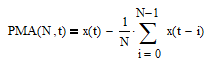
The PMA indicator is described in more detail in Section 6 of [2]. The 10-month PMA indicator generates the same trading signals as the 10-month MA filter when the PMA indicator output crosses above (buy) or below (sell) zero.

The 10-month PMA indicator coefficients are shown in the following graph.

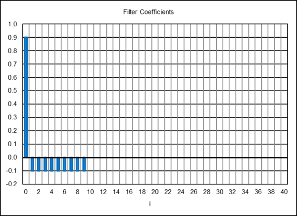
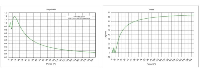
Using the PMA indicator coefficients with a digital filter design and analysis tool confirms that the 10-month PMA indicator is a high pass FIR filter with a -3 dB cutoff period P_c of approximately 37 months, as shown the left-hand graph below. The -3 dB cutoff occurs at the period at which the filter output magnitude crosses the √½ = 0.7071 level (see Section 2 of [2] for the calculation details). The phase response of the indicator is shown in the right-hand graph.

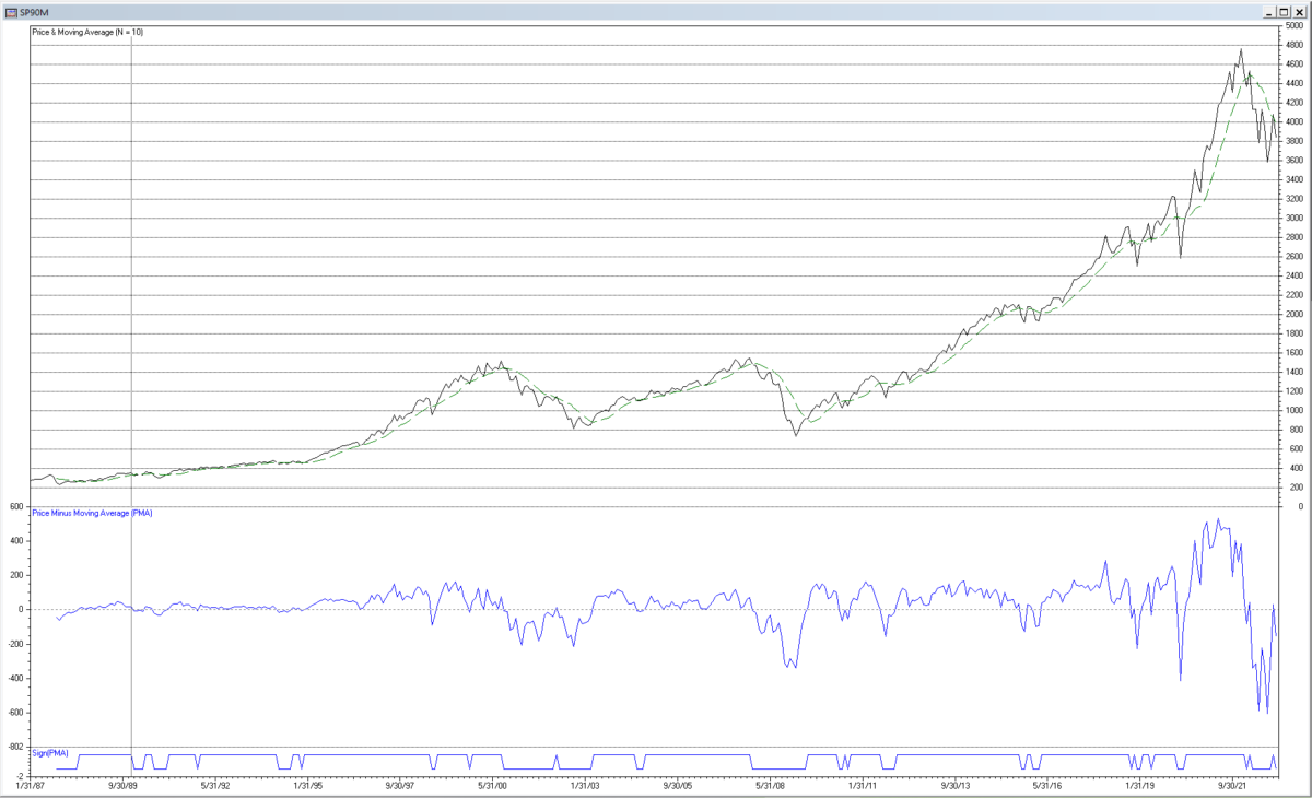
The chart below shows the 10-month PMA indicator applied to the monthly S&P 500 index for the years 1990 to 2022. PMA trading signals are generated in the time domain when the PMA indicator output crosses above (buy) or below (sell) zero, as indicated by the line at the bottom of the chart.

5.    12-Month Time Series Momentum

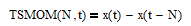
The 12-month time series momentum (TSMOM) indicator was documented as a significant “smart beta” investment factor in a paper by Tobias Moskowitz, Yao Hua Ooi, and Lasse Pederson [5] and is often used as an alternative to the 10-month MA indicator. The TSMOM indicator calculates the difference between two data points that are separated by a fixed number of integer time samples, called the lookback, and is the simplest FIR differentiator. The TSMOM indicator equation with a lookback of N time samples is:

The TSMOM indicator is described in more detail in Section 12 of [2].

MA and TSMOM are mathematically related (see Section 12 of [2] for the derivation). The relation of a TSMOM indicator with lookback N to a MA filter of length N is:

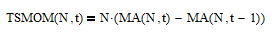
As indicated by this relation, TSMOM with lookback N is the scaled difference between the value of a MA filter of length N at time t and its value at time t-1. Thus, in the time domain, TSMOM changes sign when the corresponding MA filter output passes an inflection point, i.e., changes direction.

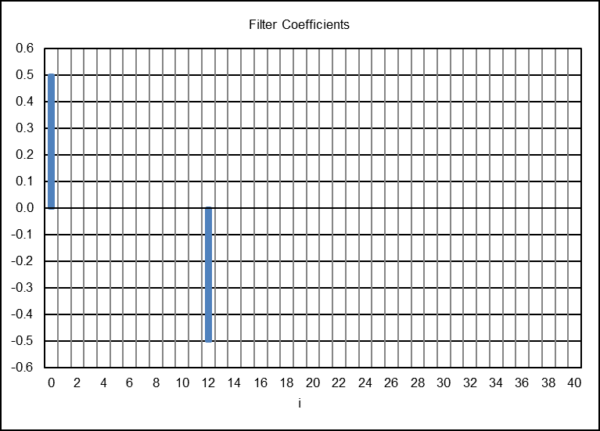
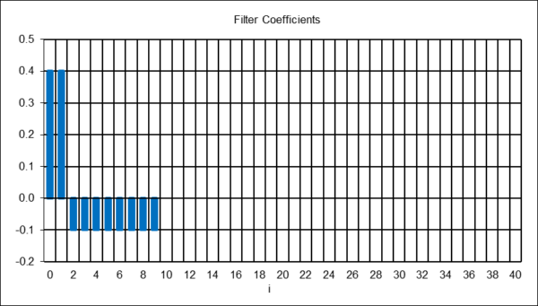
The gain-adjusted 12-month TSMOM indicator coefficients are shown below, where the standard TSMOM indicator coefficients are divided by b(0) = 2, resulting in a gain factor of 0.5, so that the maximum magnitude response of the indicator is set to 1.0 (0 dB).

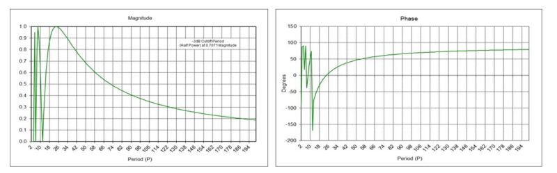
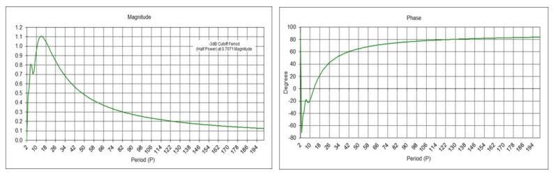
Using the gain-adjusted TSMOM indicator coefficients with a digital filter design and analysis tool produces the magnitude and phase responses shown below. The 12-month TSMOM indicator completely passes periods of 2.1818, 2.667, 3.4286, 4.8, 8, and 24 months and completely suppresses periods of 2, 2.4, 3, 4, 6, and 12 months. The phase response of the indicator is shown in the right-hand graph.

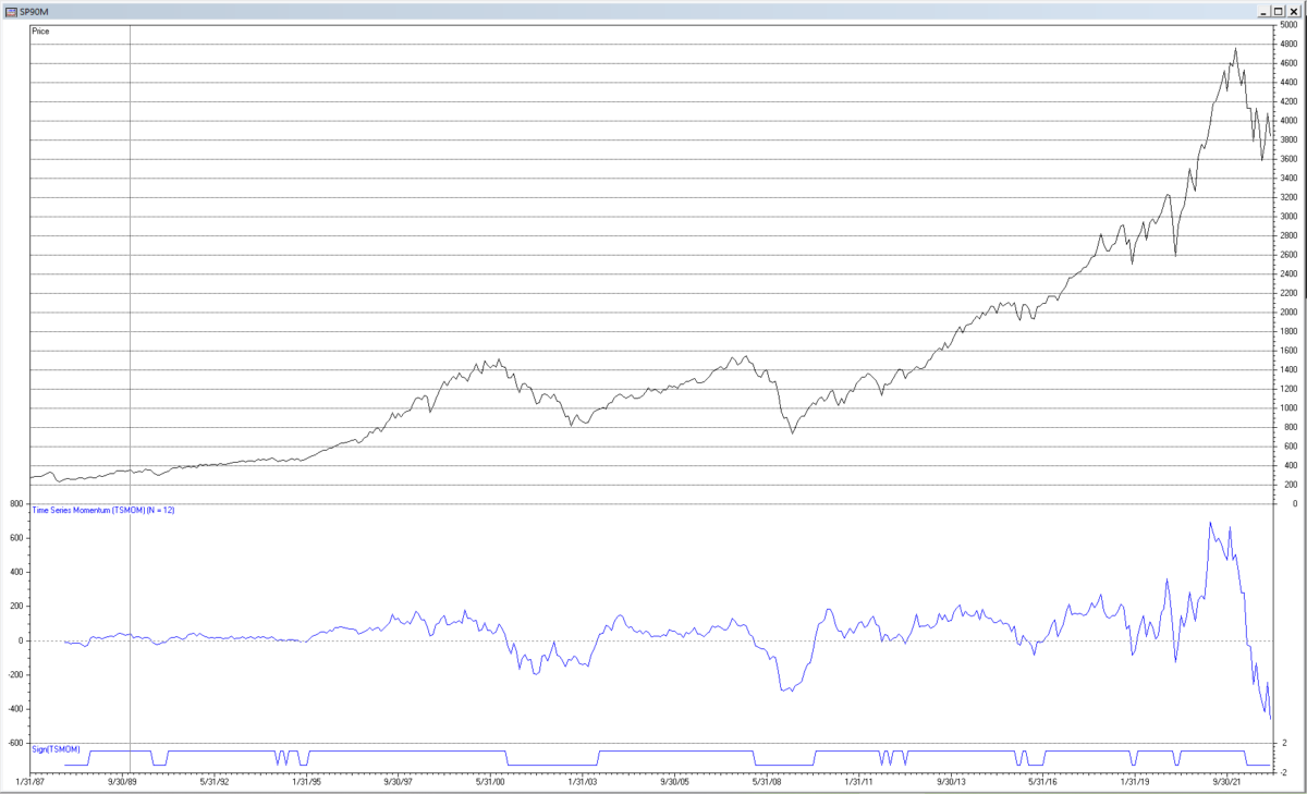
The following chart shows the 12-month TSMOM indictor applied to the monthly S&P 500 index for the years 1990 to 2022. The zero-line crossing buy and sell trading signals generated in the time domain are indicated by the line at the bottom of the chart.

6. Moving Average Crossover

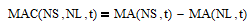
William Brock, Josef Lakonishok, and Blake LeBaron conducted one of the first detailed studies of the moving average crossover (MAC) indicator [6]. The MAC indicator uses the difference between two MAs, where one MA has a short length N_S and the other has a long length N_L with 1 < N_S < N_L. If N_S = 1, the MAC indicator reduces to the PMA indicator. The MAC indicator equation is:

The MAC indicator is described in more detail in Section 14 of [2].

MAC is a type of FIR bandpass filter, since subtracting a low pass filter with a large cutoff period from a low pass filter with a small cutoff period results in a bandpass filter. A bandpass filter passes periods between a short cutoff period P_cS and a long cutoff period P_cL, which is called the bandwidth ∆P = P_cL – P_cS, and attenuates the others. The filter has a center (also called “resonant”) period P₀, which the filter passes at maximum power. The bandwidth and center period of the MAC indicator are determined by the two MA lengths N_S and N_L.

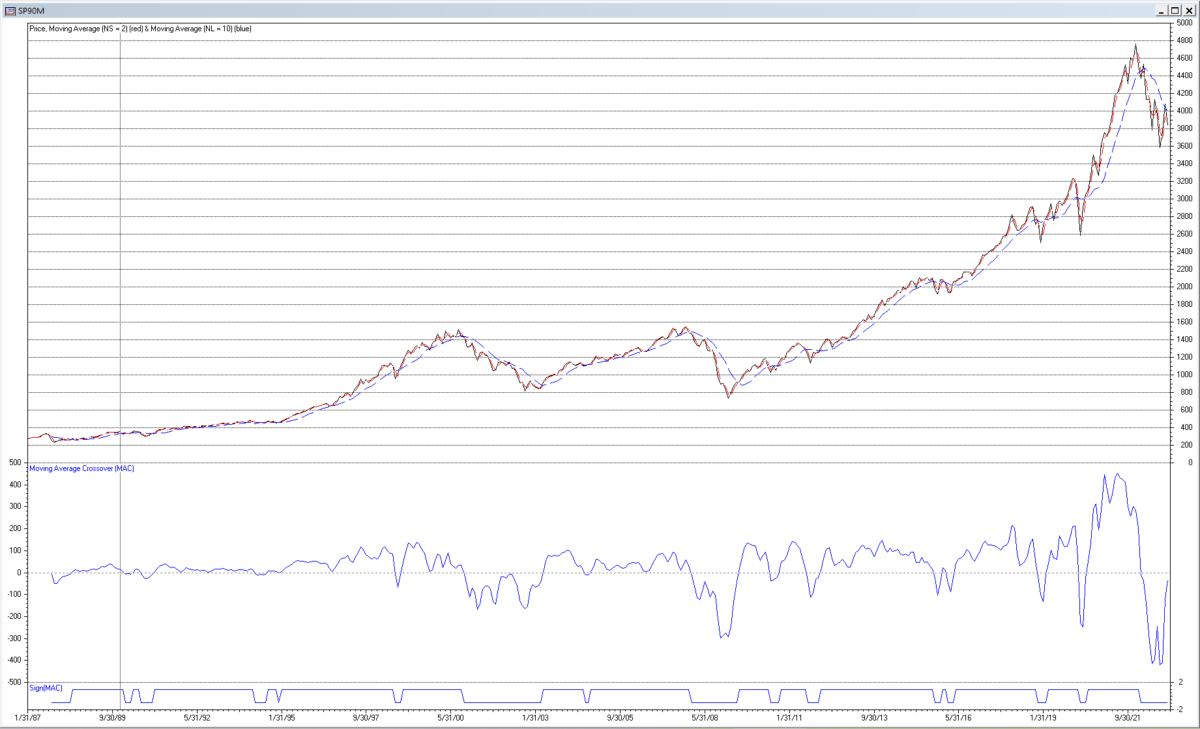
The MAC indicator was originally designed for and is commonly used with daily prices. Two popular daily MAC indicators, one called the “Golden Cross”, which is used to identify bull markets when MA(N_S, t) crosses above MA(N_L, t), and the other called the “Death Cross”, which is used to identify bear markets when MA(N_S, t) crosses below MA(N_L, t), employ a short length N_S = 50 trading days and a long length N_L = 200 trading days. While these parameters could be used with monthly prices, they can potentially generate trading signals with unacceptable delay. In this example, roughly comparable monthly MA lengths are used for illustration purposes, i.e., N_S = 2 months and N_L = 10 months, assuming 252 trading days in a year. The following graph shows the resulting MAC indicator coefficients.

Using these MAC indicator coefficients with a digital filter design and analysis tool produces the magnitude and phase responses shown below. The magnitude graph shows that the center period P₀ of the indicator is approximately 14 months. The short cutoff period P_cS is approximately 7 months, and the long cutoff period P_cL is approximately 33 months, resulting in a bandwidth ∆P of approximately 26 months. The phase response of the indicator is shown in the right-hand graph.

The following chart shows the output of the example MAC indicator applied to the monthly S&P 500 index for the years 1990 to 2022. MAC trading signals are generated in the time domain when the MAC indicator output crosses above (buy) or below (sell) zero, as indicated by the line at the bottom of the chart.

7. Moving Average Convergence-Divergence

The moving average convergence-divergence (MACD) indicator was developed by Gerald Appel in the late 1970’s (see, for example, [7] for further details). Despite the name, the MACD indicator is calculated using the difference between two exponential smoothing (ES) filters, not two MA filters. An ES filter is an IIR low pass filter. The equation of an ES filter with smoothing constant α is:

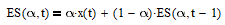
where 0 <= α <= 1. The ES filter is described in more detail in Section 9 of [2]. The cutoff period P_c of an ES filter is inversely proportional to the smoothing constant α.

MACD parameters are usually specified using MA lengths instead of smoothing constants, which are inversely proportional to MA lengths. The result is one ES, with a large smoothing constant α_L, is based on the short MA length N_S, and the other ES, with a small smoothing constant α_S, is based on the long MA length N_L. The MACD indicator equation is:

where α_L = 2/(N_S + 1), α_S = 2/(N_L + 1), 1 < N_S < N_L, and 0 < α_S < α_L <= 1. If N_S = 1, the MACD indicator reduces to the price minus exponential smoothing (PES) indicator (see Section 8 below regarding the PES indicator). The MACD indicator is described in more detail in Section 15 of [2]. While the MAC indicator is a type of FIR bandpass filter, MACD is a type of IIR bandpass filter. The bandwidth and center period of the MACD indicator are determined by the two smoothing constants α_L and α_S.

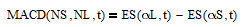
The MACD indicator was originally designed for and is commonly used with daily prices. The standard MACD indicator MA lengths are N_S = 12 trading days and N_L = 26 trading days. While these parameters could be used with monthly prices, they can potentially generate trading signals with unacceptable delay. Shorter MA lengths are used in this example for illustration purposes, specifically, N_S = 4 months and N_L = 8 months, which are equivalent at the quarter power (-6 dB) cutoff periods to smoothing constants α_L = 0.4 and α_S = 0.2222. The following graph shows the resulting MACD indicator coefficients, limited to the first 41.

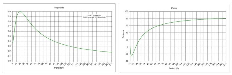
Using these MACD indicator coefficients with a digital filter design and analysis tool produces the magnitude and phase responses shown below. The magnitude graph shows that the center period P₀ of the indicator is approximately 17 months, The short cutoff period P_cS is approximately 7 months, and the long cutoff period P_cL is approximately 44 months, resulting in a bandwidth ∆P of approximately 37 months. The phase response of the indicator is shown in the right-hand graph.

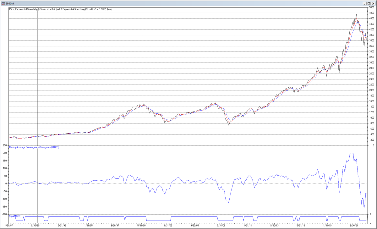
The following chart shows the output of the example MACD indicator applied to the monthly S&P 500 index for the years 1990 to 2022. MACD trading signals can be generated in the time domain in several ways. One type of trading signal is generated when ES(α_L, t) crosses above (buy) or below (sell) ES(α_S, t), which is called the “MACD line”. Another type of trading signal additionally smooths the MACD line using another ES filter to generate a “signal line”, in which case the trading signal is generated when the MACD line crosses above (buy) or below (sell) the signal line. In this example, MACD trading signals are generated when the MACD indicator output, which is the same as the MACD line, crosses above (buy) or below (sell) zero, as indicated by the line at the bottom of the chart.

8.    Markov Switching Model Rule

The Markov Switching Model rule is derived in a recent paper by Valeriy Zakamulin and Javier Giner, based on a Markov switching model of stock market states [8]. The rule results in an ES filter with decay factor λ = 0.801, as determined for the S&P 500 index. The equivalent smoothing constant is α = 1 – λ = 0.199. An ES filter with smoothing constant α = 0.199 has approximately the same quarter power (-6 dB) cutoff period as a moving average filter with length N = (2 – α)/α = 9 time samples. Trading signals are generated when the current month-end price crosses above (buy) or below (sell) the current ES filter output.

Subtracting the output of an ES filter from the current price is sometimes referred to as a price minus exponential smoothing (PES) indicator. Subtracting an IIR low pass filter from the current input results in an IIR high pass filter. The equation of a PES indicator with smoothing constant α is:

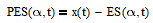
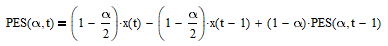
which can be rewritten as:

Adjusting the indicator gain so that the maximum magnitude response is 1.0 (0 dB) results in:

The PES indicator is described in more detail in Section 10 of [2]. The PES indicator generates the same trading signals as the Markov Switching Model rule when the PES indicator output crosses above (buy) or below (sell) zero.

The PES indicator coefficients with α = 0.199 are shown below, limited to the first 41.

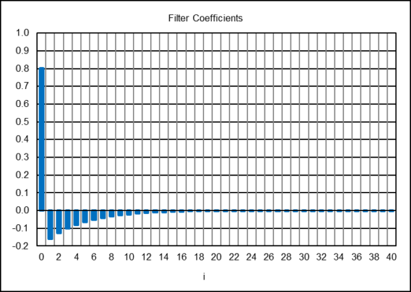
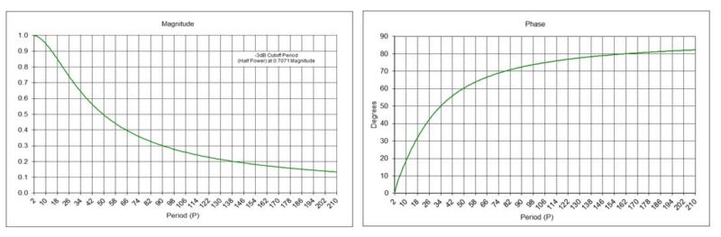
Using the PES indicator coefficients with a digital filter design and analysis tool confirms that the Markov Switching Model rule acts as an IIR high pass filter with a -3 dB cutoff period P_c of approximately 29 months, as indicated in the magnitude graph. The phase response of the indicator is shown in the right-hand graph.

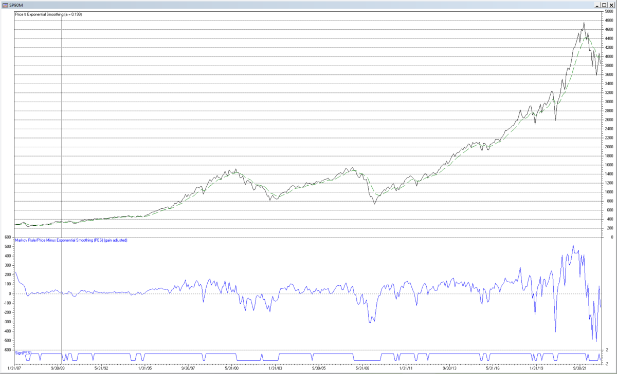
The following chart shows the output of the Markov Switching Model rule applied to the monthly S&P 500 index for the years 1990 to 2022. Buy and sell trading signals generated by the rule in the time domain are indicated by the line at the bottom of the chart.

9.    Semi-Markov Switching Model NB(4) Rule

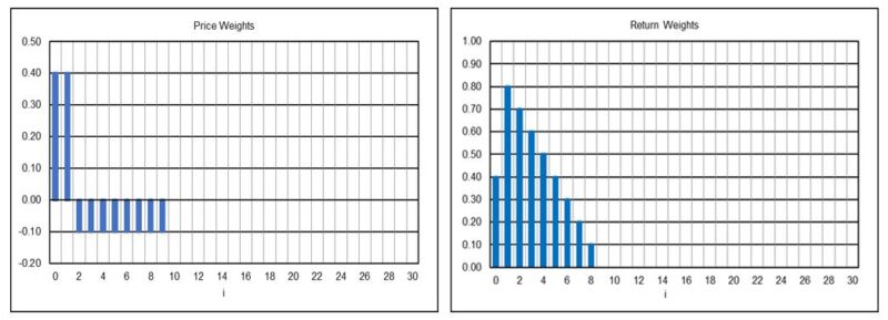
The Semi-Markov Switching Model NB(4) rule is also derived in [8], based on a semi-Markov switching model of stock market states. The rule results in a set of return weights, where return weight rw(i) is multiplied with the corresponding change in price ∆p(t-i), in contrast to multiplying filter coefficients a(i) with prices p(i), when calculating the output of an indicator. The general equation of an indicator using return weights is:

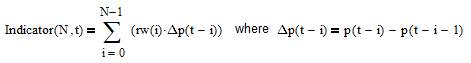
See, for example, [9] and [10] for details regarding the calculation and use of return weights when evaluating the properties of indicators.

The Semi-Markov Switching Model NB(4) rule return weights are not listed in the paper but were graciously provided by Valeriy Zakamulin, the first 30 of which are shown in the second column of the table below. The return weights are shown graphically in Appendix 3, along with those of the other indicators discussed in this article.

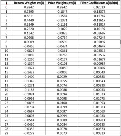
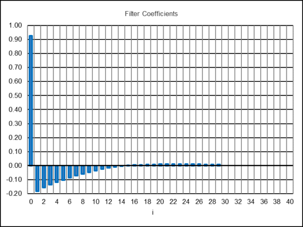
The Semi-Markov Switching Model NB(4) rule can be modeled as a truncated IIR filter. The corresponding price weights pw(i) were calculated from the return weights rw(i) using the method described in Appendix 3 and are shown in the third column of the table. The filter coefficients a(i)/b(0), where b(0) = 1, that are used with the digital filter design and analysis tool are set equal to the corresponding price weights pw(i), but because the return weights are limited to the first 30 values, the price weights do not sum to zero. As a result, the filter coefficients need to be adjusted so that they sum to zero, otherwise a bias is introduced. The adjusted filter coefficients are listed in the fourth column of the table and shown graphically below, limited to the first 30.

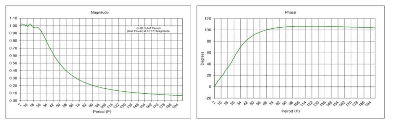
The magnitude response of the Semi-Markov Switching Model NB(4) rule, shown in the left-hand graph below, indicates that it is a FIR high pass filter with a -3 dB cutoff period P_c of approximately 38 months. The phase response of the rule is shown in the right-hand graph.

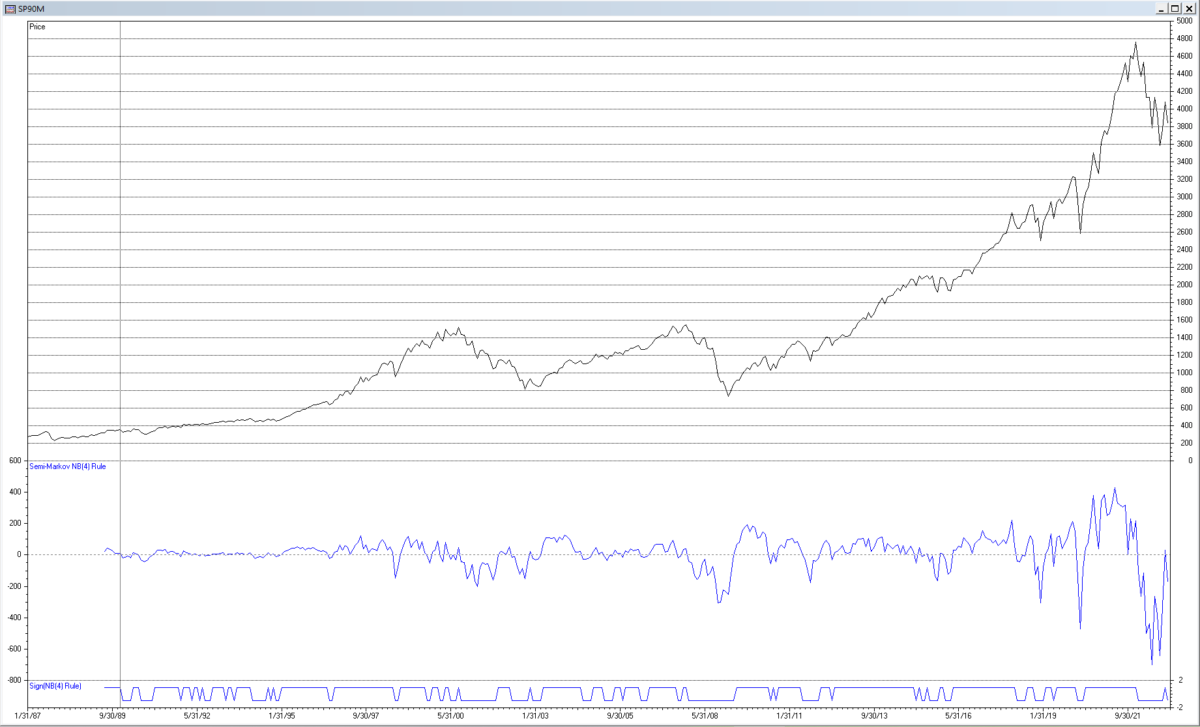
The following chart shows the Semi-Markov Switching Model NB(4) rule applied to the monthly S&P 500 index for the years 1990 to 2022. The zero-line crossing buy and sell trading signals produced by the rule in the time domain are indicated by the line at the bottom of the chart.

10. Summary

The table below summarizes the six indicators by unit pulse response, filter type, and magnitude response characteristics:

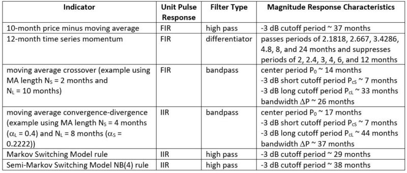
Note that the coefficients of all the indicators are fixed and do not change over time. Since financial time series are non-stationary, i.e., their return probability distributions are not invariant under time shift and cycles and trends do not persist, the use of filters with fixed parameters will not perform well at all times for trading purposes.

Acknowledgements

I would like to thank Valeriy Zakamulin for providing many helpful comments as well as providing the Semi-Markov Switching Model NB(4) rule return weights.

Appendix 1 – Frequency Response

The frequency response H(ω) of a filter to a sinusoidal input with frequency ω radians is:

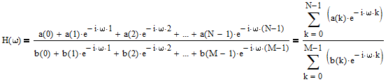
where the a(k) and b(k) are filter coefficients discussed in Section 2 and i = √-1. The magnitude response |H(ω)| is:

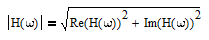
where Re(H(ω)) is the real part of H(ω) and Im(H(ω)) is the imaginary part. The phase response θ(ω) is:

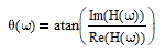
Phase response θ(ω) values can be converted from radians to degrees by multiplying by 180/π.

Appendix 2 – Discrete Fourier Transform

Digital signals and time series can be analyzed in the frequency domain using the Discrete Fourier Transform (DFT). The DFT calculation is:

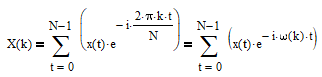
where

• N = number of samples of the signal or time series x(t)
• x(t) = signal or time series sample at integer time t = 0, 1, 2, …, N-1
• i = √-1
• X(k) = frequency component k for k = 0, 1, 2, …, N-1
• ω(k) = 2*π*k/N = frequency of frequency component X(k) in radians.

Frequency ω(k) in radians can be converted to frequency f(k) using f(k) = ω(k)/(2*π) or to period P(k) using P(k) = 2*π/ω(k).

The amplitude |X(k)| of frequency component k is:

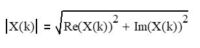
where Re(X(k)) is the real part of X(k) and Im(X(k)) is the imaginary part of X(k). The phase θ(X(k)) of frequency component k in radians is:

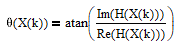
Phase response θ(X(k)) values can be converted from radians to degrees by multiplying by 180/π.

Appendix 3 – Price Weight and Return Weight Calculation

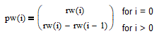
The general equations used to calculate price weights from return (i.e., price change) weights and return weights from price weights are:

1. Price weights – Price weights pw(i) can be calculated from return weights rw(i) using the following differencing equation:

2. Return weights – Return weights rw(i) can be calculated from price weights pw(i) using the following summation equation:

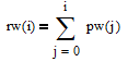
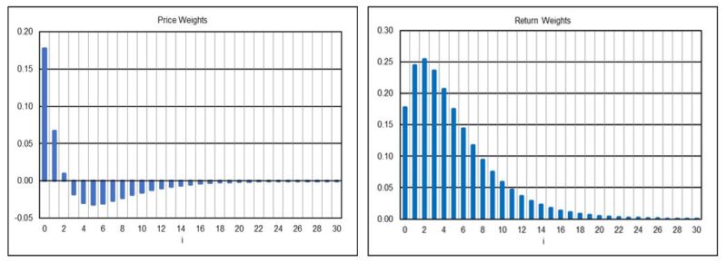
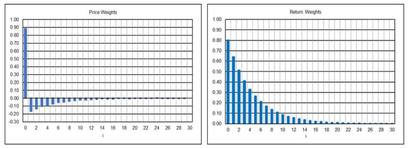
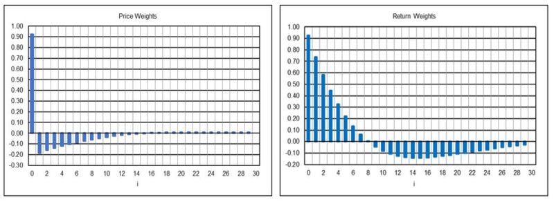
The following graphs show the price weights pw(i), which are equivalent to filter coefficients a(i), and the corresponding return weights rw(i) for the six indicators discussed in this article.

10-Month Price Minus Moving Average (N = 10)

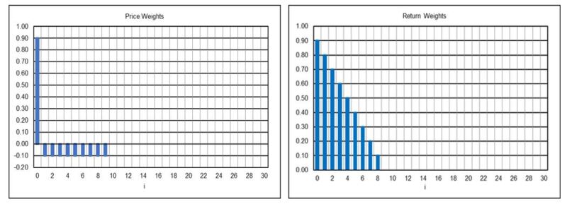
12-Month Time Series Momentum (N = 12) (gain-adjusted)

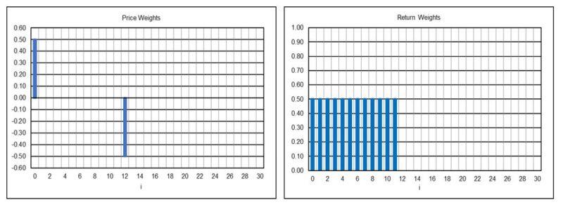
Moving Average Crossover (N_S = 2, N_L = 10)

Moving Average Convergence-Divergence (α_S = 0.2222, α_L = 0.4)

Markov Switching Model Rule (Price Minus Exponential Smoothing with α = 0.199)

Semi-Markov Switching Model NB(4) Rule (weights limited to the first 30)

References

[1] Oppenheim, A. V., Willsky, A. S., and Young, I. T., Signals and Systems, Prentice Hall, 1983.

[2] Stern, H., “An Introduction to Digital Signal Processing for Trend Following”, August 2020; available online at https://alphaarchitect.com/2020/08/an-introduction-to-digital-signal-processing-for-trend-following/.

[3] Delgutte, B. and Greenberg, J., Biomedical Signal and Image Processing, Chapter 4 – The Discrete Fourier Transform, 1999; available online at https://web.mit.edu/~gari/teaching/6.555/lectures/ch_DFT.pdf, 2005.

[4] Faber, M. T., “A Quantitative Approach to Tactical Asset Allocation”, The Journal of Wealth Management, Spring 2007; available online at http://ssrn.com/abstract=962461.

[5] Moskowitz, T. J., Ooi, Y. H., and Pedersen, L. H., “Time Series Momentum”, Journal of Financial Economics, 104 (2), 228-250, May 2012; available online at http://docs.lhpedersen.com/TimeSeriesMomentum.pdf.

[6] Brock, W., Lakonishok, J., and LeBaron, B., “Simple Technical Trading Rules and the Stochastic Properties of Stock Returns”, The Journal of Finance, 47 (5), 1731-1764, December 1992; available online at https://www.santafe.edu/research/results/working-papers/simple-technical-trading-rules-and-the-stochastic-.

[7] Appel, G. and Dobson, E., Understanding MACD (Moving Average Convergence Divergence), Traders Press Inc., 2008.

[8] Zakamulin, V. and Giner, J., “Optimal Trend Following Rules in Two-State Regime-Switching Models”, September 2022; available online at https://papers.ssrn.com/sol3/papers.cfm?abstract_id=4217513.

[9] Levine, A. and Pedersen, L. H., “Which Trend is Your Friend?”, Financial Analysts Journal, 72 (3), 51-66, May/June 2016; available online at https://papers.ssrn.com/sol3/papers.cfm?abstract_id=2603731.

[10] Zakamulin, V., Market Timing with Moving Averages: The Anatomy and Performance of Trading Rules, Springer, 2017.