Investors are enamored with various investment houses and personalities who claim insight into the prospects for return forecasting. Some classic examples include Nouriel Roubini, John Hussman, David Rosenberg, or Jeremy Grantham. All really smart people.
But have you ever asked “How” these folks came to their conclusions?
In most cases, the answer is probably “No” and the reason is because there is a lack of transparency from the author(s) and/or a lack of knowledge/understanding on behalf of the reader. We also want to highlight that one can develop incredibly complex return forecasting models — super sexy, super interesting, super compelling, etc. — but that still doesn’t mean they are any good at forecasting much of anything.
The point of this learning module is to educate the reader so they can make informed decisions about long-term expected return forecasting models. (1)
A PDF version of this is available here.
Summary of Return Forecasting models
We generate projected long-term expected return forecasts for the S&P 500 using a variety of models ranging from simple (Bob Shiller Method) to medium complexity (Hussman Method) to relatively complex (Alpha Architect Method).
Core model inputs are as follows:
- Current P/E: 18.10 (As of 7/7/2014)
- Current Profit Margin: 13.35% (As of 7/7/2014)
- Current Cyclically Adjusted Price/Earnings (CAPE or Shiller P/E): 25.82 (As of 6/30/2014)
Shiller Method (Simple)
- Regression approach
- The current predicted 10-year Nominal Total Return: 6.06%.
Hussman Method (mid range complexity)
- Total return approach with assumptions on exit valuations.
- The current predicted 10-year nominal total return ranges between: -4.16% and 5.52%.
Alpha Architect Method (high complexity)
- Simulation approach with dynamic revenue, profit margins, and valuations.
- The current predicted 10-year nominal total return ranges between: 3.42% and 5.49%.
- The top line is with average/good input assumptions.
- The bottom line is with below average/poor input assumptions.
The results are hypothetical results and are NOT an indicator of future results and do NOT represent returns that any investor actually attained. Indexes are unmanaged, do not reflect management or trading fees, and one cannot invest directly in an index. Additional information regarding the construction of these results is available upon request.
Generating Expected Real Return Forecasts
Shiller Method (simple)
We identify two variables:
- The cyclically adjusted PE yield (1/CAPE) for any given point in time.
- The subsequent 10 year average total returns (nominal) from that date.
Next, we run a regression on these two variables, using input from 1/31/1881 through 9/30/2001 and solve for an intercept, A, and a slope, B, in the regression equation Y = A + BX + error. Then we get the following estimated regression equation:
- 10-year Nominal Total Return=0.9198495*(1/CAPE)+0.024967
- A detailed explanation can refer to an earlier post here: The Shiller P/E Ratio.
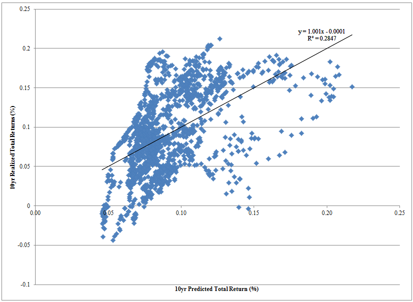
The figure below highlights the relationship between actual 10-year realized return observations and predicted 10-year returns using the simple Shiller prediction model.
The results are hypothetical results and are NOT an indicator of future results and do NOT represent returns that any investor actually attained. Indexes are unmanaged, do not reflect management or trading fees, and one cannot invest directly in an index. Additional information regarding the construction of these results is available upon request.
This model is estimated “in-sample” meaning that the usefulness of the regression estimates are only useful to the extent that one believes the historical linear relationship between 1/CAPE and future returns remains constant “out of sample.”
- The current predicted 10-year Nominal Total Return: 6.06% (As of 6/30/2014, CAPE=25.82, plug it into the equation above)
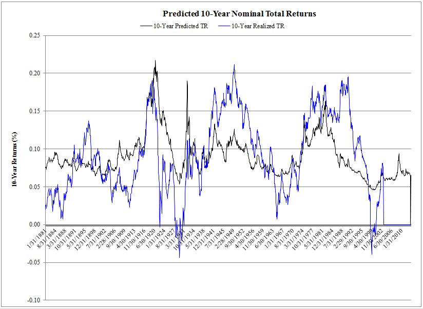
- Below we plot the 10-year predicted total return using the Shiller Method and the realized 10-year total return.
The results are hypothetical results and are NOT an indicator of future results and do NOT represent returns that any investor actually attained. Indexes are unmanaged, do not reflect management or trading fees, and one cannot invest directly in an index. Additional information regarding the construction of these results is available upon request.
The figure above plots the relationship between actual 10-year realized return observations and predicted 10-year returns using the simple Shiller prediction model.
The Shiller model does a decent job predicting the general movement of future returns, but realized returns are much more volatile than those predicted by the Shiller model. Plus, this model is really simple.
Hussman Method (mid-level complexity)
Background article on the Hussman Method: Long-term Market Return Projections
Philosophical Economics has some additional thoughts on the validity of this approach (and the Hussman rebuttal), but we aren’t here to highlight which model is good or bad, rather, we are simply showing the reader how they are created.
In the short piece Hussman suggests that the projected annual total return on the S&P 500 over T years can be represented with the following equation:
- Long term total return = (1+g)(future CAPE / current CAPE)^(1/T) – 1 + dividend yield(current CAPE / future CAPE + 1) / 2
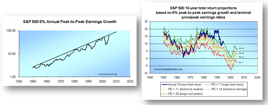
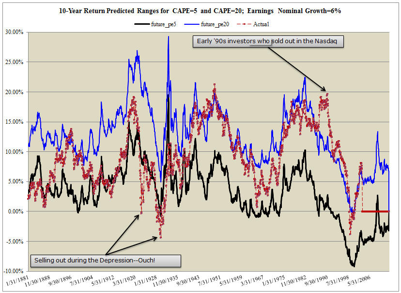
We make the following assumptions and plug them into the equation above:
- Peak to Peak earnings growth, g=6%
- T=10 years
- Dividend yield = 2.24%
- Current CAPE = 25.82 (as of 6/30/2014)
- future CAPE (E=Peak Earnings over cycle) range between 20 (major bull) and 5 (major bear)
The current predicted 10-year nominal total return ranges between: -4.16% and 5.52%.
The results are hypothetical results and are NOT an indicator of future results and do NOT represent returns that any investor actually attained. Indexes are unmanaged, do not reflect management or trading fees, and one cannot invest directly in an index. Additional information regarding the construction of these results is available upon request.
The figure above highlights 10-year predict total return ranges under different ending valuations regimes. The “worst-case” regime is a CAPE = 5 (black line) and the “best-case” regime is a CAPE = 20 (blue line). We also plot realized 10-year total returns to assess how well the upper and lower ranges have captured historical realized return measures.
This model is effective at pinpointing the potential ranges for future returns, at least historically. There are a few notable exceptions, such as the Great Depression and the Internet Bubble. Outside of these rare events, one can reasonably expect future 10-year returns to fall within the bounds predicted by this model.
Alpha Architect Method (way too complex)
Both the Shiller and the Hussman method for predicting long-term returns suffer from an inability to effectively model parameters that matter to future returns. For example, the Hussman model makes an assumption of 6% peak to peak earnings growth. But is this a reasonable assumption if profit margins are at all-time highs and known to mean-revert?
A more sophisticated model might be needed.
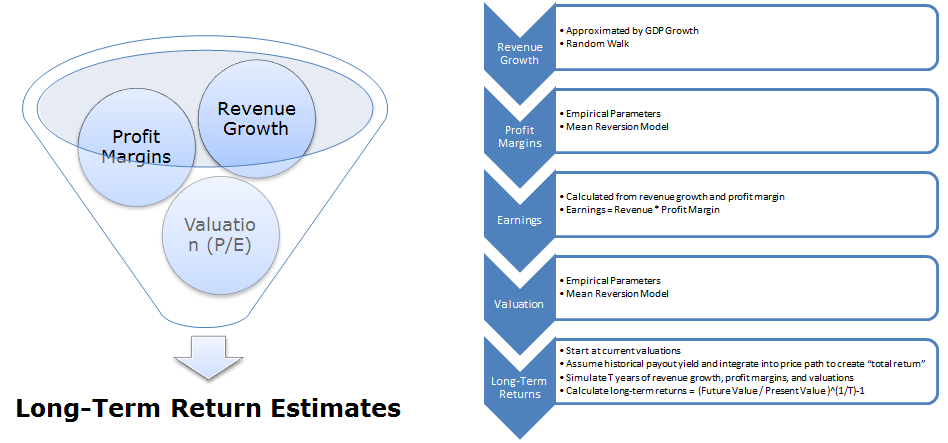
Our approach to this problem begins with a 40,000 foot view of the drivers of long-term returns:
- Revenue growth
- Margins
- Valuations
Any long-term return projection models needs to account for the empirically-observed dynamics of these variables.
- Revenue growth
- In particular, revenue growth (as approximated by GDP) follows a fairly stable growth pattern, but with bumps along the road. We model this “bump” aspect by simulating growth paths at a static growth rate, but add a random volatility component around this static growth rate.
- Margins
- For profit margins, the dynamic is a bit different. Margins tend to mean-revert, in other words, currently high margins systematically drift back to the long-term average and currently low margins drift up to the long-term average. This mean-reversion reflects the competitive dynamics in the economy.
- Valuations
- Finally, valuations are modeled in a similar fashion to margins—mean-reverting. Higher valuations are typically not followed with even higher valuations in the future (unless we are reliving the Internet Bubble).
Here is the breakdown of the process:
- Estimate Nominal Revenue Growth as a growing, but volatile time series.
- Estimate Margins as a mean-reverting, but volatile time series.
- Revenues + Margins –>Generate Earnings
- Estimate Valuations as a mean-reverting, but volatile time series.
- Estimate Payout Ratios—we just use the historical average and assume this stays in place in the future.
- Earnings + Payout Ratio + Valuation –> Generate total expected return forecasts
First, an Introduction to some Basic Modeling Techniques
Let’s first introduce some basic modeling techniques:
- Random walks
- Mean reverting processes.
Random Walk:
We model GDP, or revenue growth, such that GDP tomorrow is equal to GDP today, plus an element of normally distributed randomness surrounding a mean expected growth rate.

Example: GDP was $10 this year. Average GDP growth is 3% and the standard deviation of GDP growth is 4%.
- Generate Random Normal Variable~(3%,4%); say, 4.26% (good year)
- GDP next year will be $10*(1+.0426)=$10.426
- Generate Random Normal Variable~(3%,4%); say, -1.0% (bad year)
- GDP twos years from now will be $10.426*(1-.01)=$10.32174
Mean Reversion Process:
We model profit margins and valuations as mean-reverting processes. We use the Ornstein-Uhlenbeck Process.
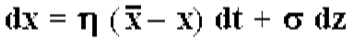
The velocity of the reversion process is a parameter in this model
- Velocity of reversion measures, “How fast it gets back to the long-term average?”
- We use a value of .2 in our models gives a half-life of 3.47 years, in other words, a observation above the long-term mean can expect to be half-way back to the mean within 3.47 years, on average.
Next, the Step by Step Process
First, let’s outline the long-term expected return forecasting framework in the graphic below:
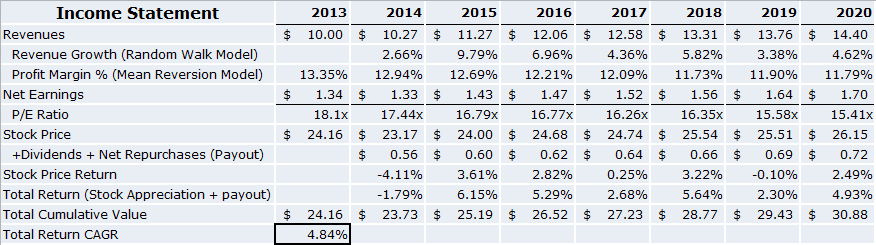
The end state of this process is to build the income statement for the economy:
The results are hypothetical results and are NOT an indicator of future results and do NOT represent returns that any investor actually attained. Indexes are unmanaged, do not reflect management or trading fees, and one cannot invest directly in an index. Additional information regarding the construction of these results is available upon request.
The income statement above is meant for illustrative purposes only. The starting values for revenues, margins, P/E, and stock price are simply initial values. The future revenue growth, profit margins, and P/E ratios are estimates from a single simulation run of the economy. To generate robust estimates for potential total returns in the future, we could run 1,000 economic simulations.
Let’s walk through the process:
Step 1: Real Revenue Growth:
Estimating Real Revenue Growth:
- S&P 500 Revenue Growth
- Approximated by real GDP growth over the long haul
- Follows a random walk with drift
- Requires initial value
- Requires initial GDP Growth Rate
- Requires estimation of GDP volatility
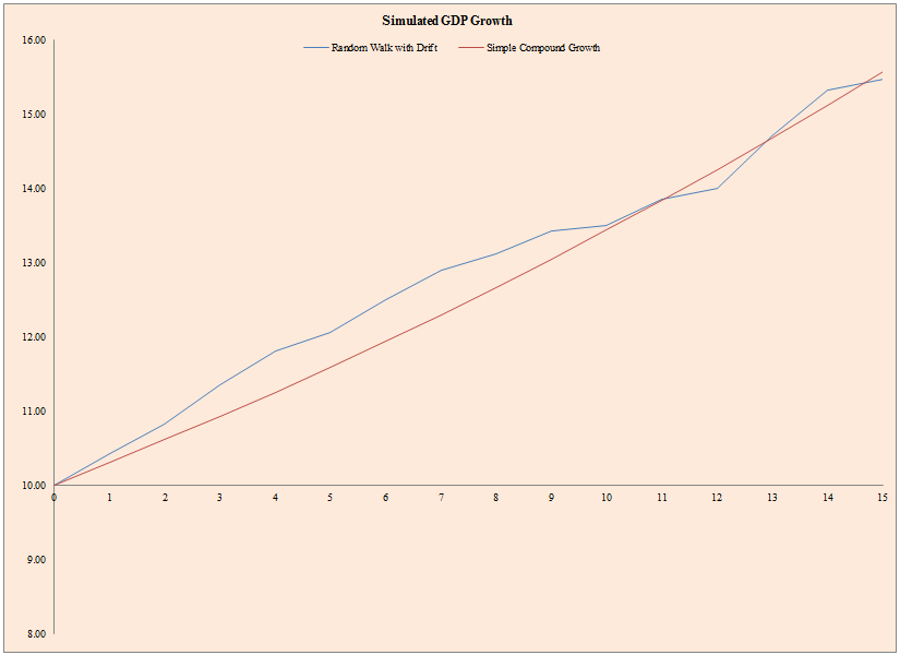
The results are hypothetical results and are NOT an indicator of future results and do NOT represent returns that any investor actually attained. Indexes are unmanaged, do not reflect management or trading fees, and one cannot invest directly in an index. Additional information regarding the construction of these results is available upon request.
- The figure above represents a single simulation of future GDP growth (blue line) and a stable GDP growth with no volatility (red line).
- The figure below shows the data that went into this chart.
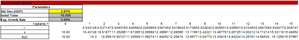
The results are hypothetical results and are NOT an indicator of future results and do NOT represent returns that any investor actually attained. Indexes are unmanaged, do not reflect management or trading fees, and one cannot invest directly in an index. Additional information regarding the construction of these results is available upon request.
But how do we figure out which parameters to use in the figures above?
Legions of economists will all have a different answer to this question, but we highlight some empirical observations and thoughts that might help one identify the “correct” parameters to plug into the model.
What has GDP looked like historically?
- The figure below plots historical GDP growth rates for different GDP time series from 1947 to 2012.
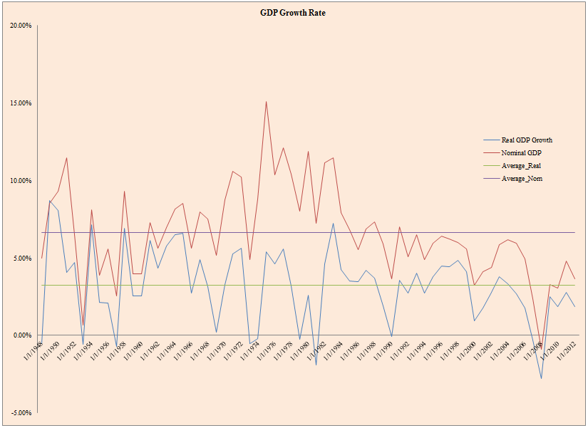
The results are hypothetical results and are NOT an indicator of future results and do NOT represent returns that any investor actually attained. Indexes are unmanaged, do not reflect management or trading fees, and one cannot invest directly in an index. Additional information regarding the construction of these results is available upon request.
- The figure below plots cumulative nominal GDP growth and real GDP growth from 1947 to 2012.
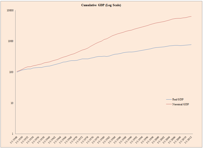
The results are hypothetical results and are NOT an indicator of future results and do NOT represent returns that any investor actually attained. Indexes are unmanaged, do not reflect management or trading fees, and one cannot invest directly in an index. Additional information regarding the construction of these results is available upon request.
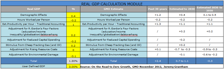
One framework for projecting future GDP
- GMO presents a basic tool to estimate potential GDP growth in the future depending on one’s assumptions for different parameters.
- We are somewhat agnostic on GDP growth over the next 30 years, but believe GMO underestimates the benefits of cheap energy and technological progress.
- GMO’s Forecast = Thomas Malthus’ Forecast = Wrong.
- Regardless, the framework below might be helpful for those pontificating the future.
How about inflation? Also a critical input for estimating nominal GDP, or revenue growth, in the future.
- The figure below plots CPI growth from 1947 to 2012.
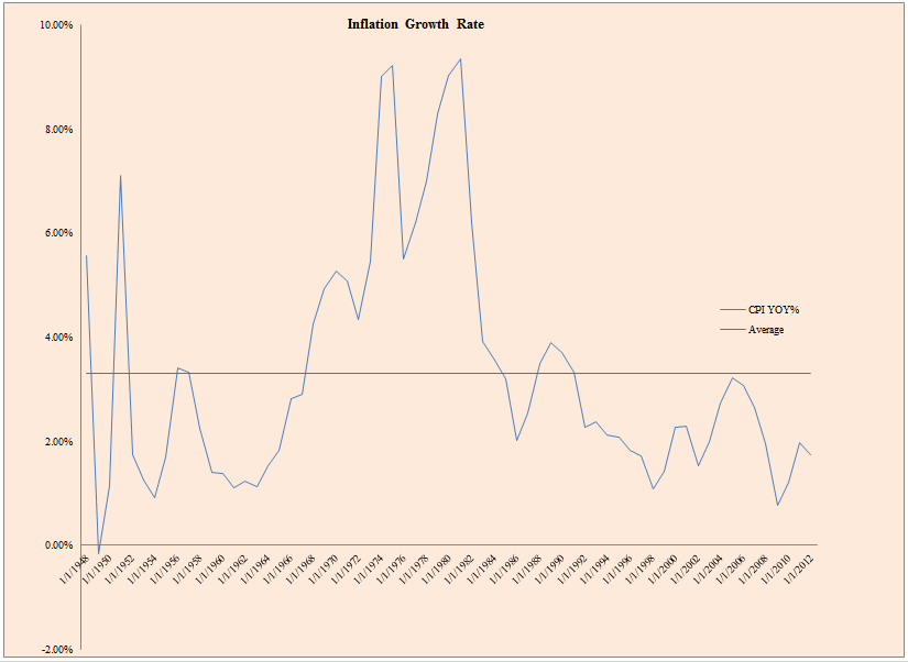
The results are hypothetical results and are NOT an indicator of future results and do NOT represent returns that any investor actually attained. Indexes are unmanaged, do not reflect management or trading fees, and one cannot invest directly in an index. Additional information regarding the construction of these results is available upon request.
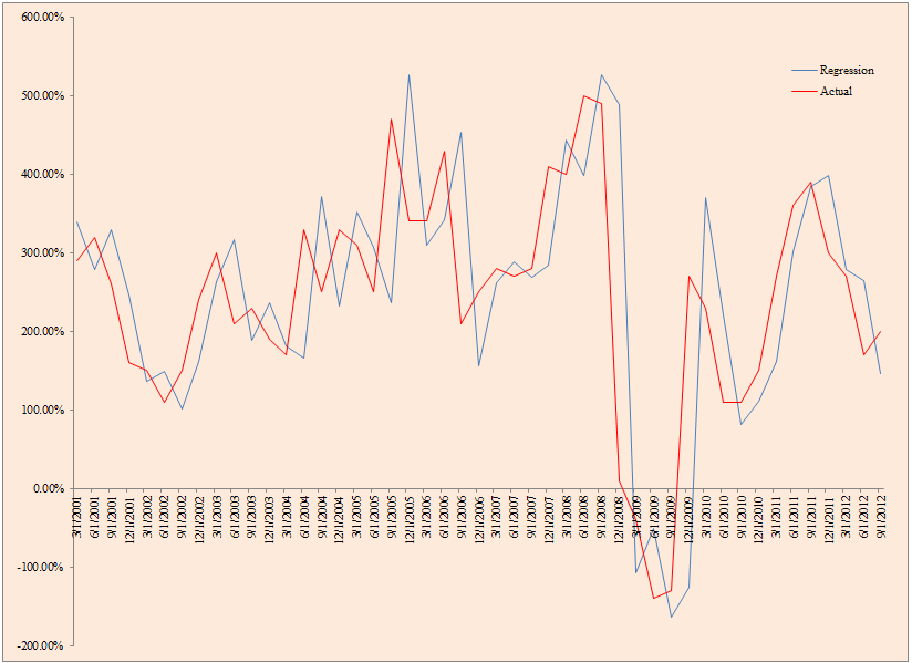
- The figure below plots realized and predicted CPI growth from 1947 to 2012.
- Our CPI forecasting method is based on a simple autoregressive framework described here.
- The chart below suggests that it is fairly accurate at predicting inflation.
The results are hypothetical results and are NOT an indicator of future results and do NOT represent returns that any investor actually attained. Indexes are unmanaged, do not reflect management or trading fees, and one cannot invest directly in an index. Additional information regarding the construction of these results is available upon request.
The inputs for revenue growth standard deviation and growth rate into the random walk simulation model mentioned at the beginning of this section, can be difficult, but perhaps the empirical figures above help guide a forecaster in the right direction.
Step 2: Profit Margins
Once we’ve identified the economy’s top line growth and revenue projections, we need to figure out how much of the revenue the “shareholders” will get to keep. In other words, the margins.
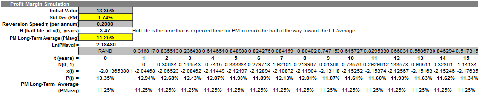
We simulate S&P 500 Profit Margins using the following framework:
- Follows a mean reversion model
- Requires initial value
- Requires profit margin volatility
- Requires mean reversion speed parameter
- Requires long-term profit margin average
- The mean reversion model simulates future profit margins that mean revert to the long-term average, albeit in a random fashion.
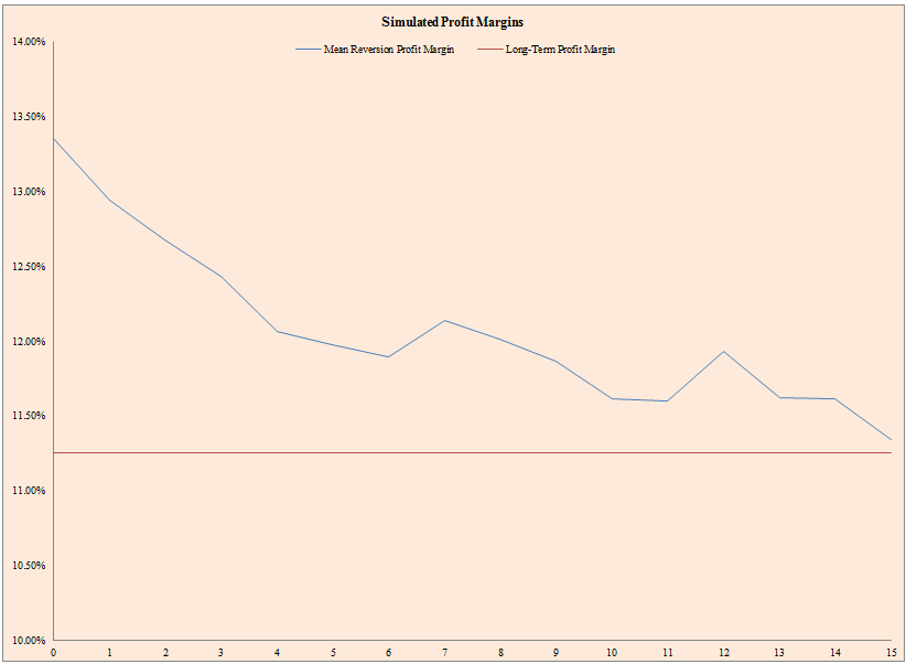
The results are hypothetical results and are NOT an indicator of future results and do NOT represent returns that any investor actually attained. Indexes are unmanaged, do not reflect management or trading fees, and one cannot invest directly in an index. Additional information regarding the construction of these results is available upon request.
- The figure above represents a single simulation of future profit margins (blue line) and average profit margins (red line). Notice that because margins are above trend, they trended down to the average in this simulation, but the ride down was bumpy and unpredictable.
- The figure below shows the data that went into this chart.
The results are hypothetical results and are NOT an indicator of future results and do NOT represent returns that any investor actually attained. Indexes are unmanaged, do not reflect management or trading fees, and one cannot invest directly in an index. Additional information regarding the construction of these results is available upon request.
But how do we figure out which parameters to use in the figures above?
Everyone has an opinion on profit margins, where they are, and where they are going. Below we present some empirical evidence to give context so one can input the right values into the profit margin simulation exercise highlighted above.
- The figure below plots realized profit margins from 2/28/1990 to 10/31/2012.
- Margins generally follow a random mean-reverting process.
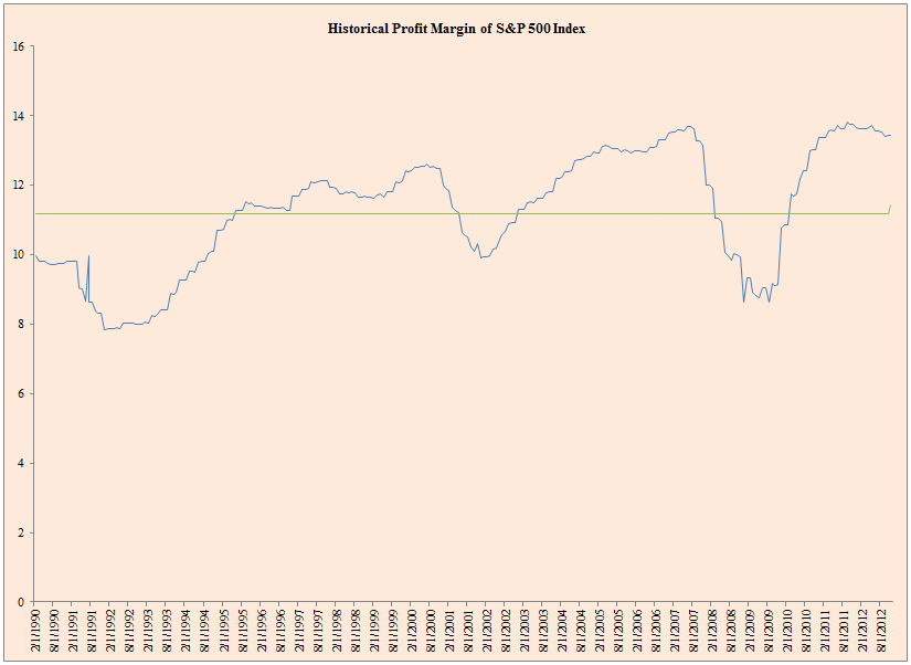
The results are hypothetical results and are NOT an indicator of future results and do NOT represent returns that any investor actually attained. Indexes are unmanaged, do not reflect management or trading fees, and one cannot invest directly in an index. Additional information regarding the construction of these results is available upon request.
Step 3: Earnings
Once we identify revenue and profit margins, calculating the earnings for the economy is straight forward:
S&P 500 Simulated Earnings = Simulated Revenue * Simulated Profit Margin
- Simulated Revenue = Nominal GDP generated via Random Walk
- Simulated Profit Margin = Profit Margin generated via mean reversion model
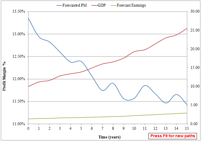
The results are hypothetical results and are NOT an indicator of future results and do NOT represent returns that any investor actually attained. Indexes are unmanaged, do not reflect management or trading fees, and one cannot invest directly in an index. Additional information regarding the construction of these results is available upon request.
- The figure above represents a single simulation of future profit margins (blue line), future revenue growth (red line), and forecasted earnings (derived from simulation of margins and revenue growth using the techniques discussed previously).
What do earnings look like historically?
Below we present some empirical evidence on historical earnings growth for the market.
- The figure below plots realized EPS growth from 1955 to 2013.
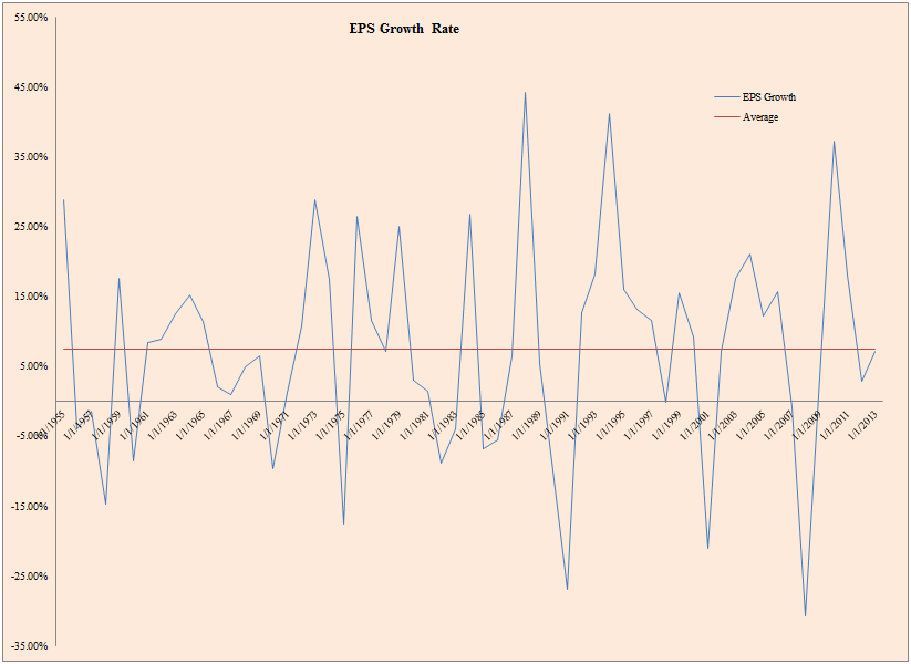
The results are hypothetical results and are NOT an indicator of future results and do NOT represent returns that any investor actually attained. Indexes are unmanaged, do not reflect management or trading fees, and one cannot invest directly in an index. Additional information regarding the construction of these results is available upon request.
Step 4: Valuation
With a projected earnings path we can identify how stock prices might move, however, we need one more piece for the puzzle: valuations.
We model valuations using the following framework:
S&P 500 Valuations (E/P)
- Follows a mean reversion model
- Requires initial value
- Requires valuation volatility
- Requires mean reversion speed parameter
- Requires long-term valuation average
- The mean reversion model simulates future valuations that mean revert to the long-term average, albeit in a random fashion.
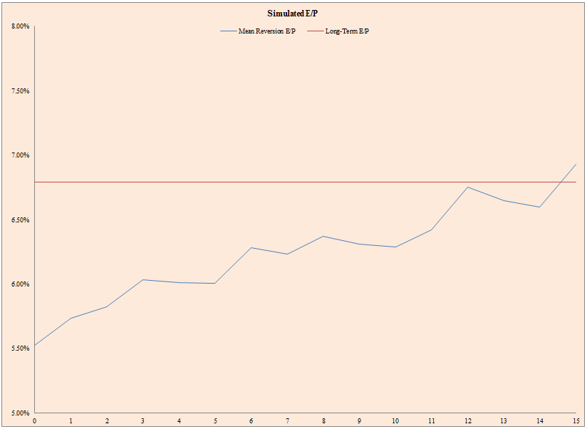
The results are hypothetical results and are NOT an indicator of future results and do NOT represent returns that any investor actually attained. Indexes are unmanaged, do not reflect management or trading fees, and one cannot invest directly in an index. Additional information regarding the construction of these results is available upon request.
- The figure above represents a single simulation of future valuations (blue line) and average valuations (red line).
- The figure below shows the inputs for the figure above.
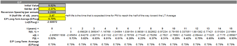
Click to enlarge. The results are hypothetical results and are NOT an indicator of future results and do NOT represent returns that any investor actually attained. Indexes are unmanaged, do not reflect management or trading fees, and one cannot invest directly in an index. Additional information regarding the construction of these results is available upon request.
But how do we figure out which parameters to use in the figures above?
Everyone has an opinion on valuations, but what do the data say on the matter?
What have valuations looked like historically?
- The figure below plots realized TTM E/P from 1955 to 2013.
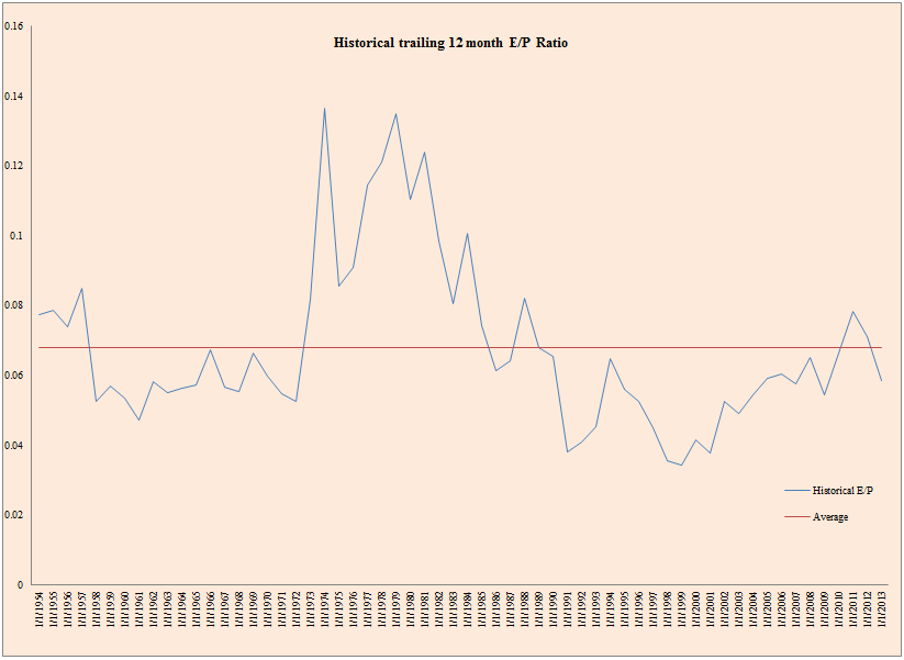
The results are hypothetical results and are NOT an indicator of future results and do NOT represent returns that any investor actually attained. Indexes are unmanaged, do not reflect management or trading fees, and one cannot invest directly in an index. Additional information regarding the construction of these results is available upon request.
Step 5: Long-Term Total Returns
After creating the economy wide balance sheet, forecasting the long-term expected returns for the stock market is a fairly easy exercise.
A recap of the process works:
- Generate simulated earnings path
- Generate simulated valuation path
- Generate simulated price path
- Estimate payout yield (dividends plus net repurchases)
- Estimate long-term returns
- (FV/PV)^(1/T)-1
- The figure above represents a single simulation of future total returns (blue line) and price-only returns (red line).
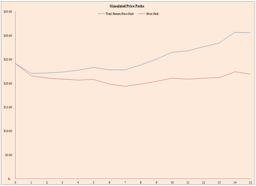
The results are hypothetical results and are NOT an indicator of future results and do NOT represent returns that any investor actually attained. Indexes are unmanaged, do not reflect management or trading fees, and one cannot invest directly in an index. Additional information regarding the construction of these results is available upon request.

The results are hypothetical results and are NOT an indicator of future results and do NOT represent returns that any investor actually attained. Indexes are unmanaged, do not reflect management or trading fees, and one cannot invest directly in an index. Additional information regarding the construction of these results is available upon request.
One element we’ve introduced above is the payout yield, which is an important component to total returns on the stock market.
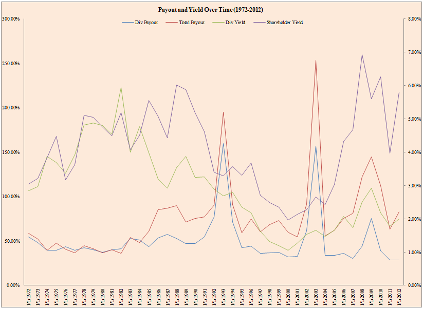
- The figure below plots dividend and net repurchases from 1972 to 2012 for S&P 500 firms (excluding financials).
- Div Payout is dividends / net income, Total Payout is dividends + net repurchases / net income, Div yield is dividends / market capitalization, and shareholder yield is dividends + net repurchases / market capitalization.
- Median Dividend Payout % is 42.26% (total dividends relative to total net income)
The results are hypothetical results and are NOT an indicator of future results and do NOT represent returns that any investor actually attained. Indexes are unmanaged, do not reflect management or trading fees, and one cannot invest directly in an index. Additional information regarding the construction of these results is available upon request.
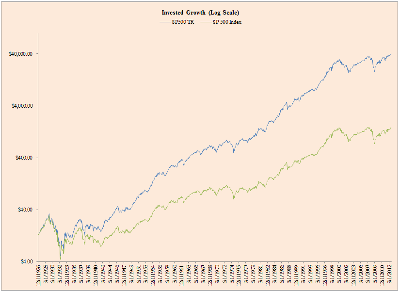
What does the historical total return and price-only return look like historically?
- The figure below plots total returns and price-only returns from 1926 to 2012.
The results are hypothetical results and are NOT an indicator of future results and do NOT represent returns that any investor actually attained. Indexes are unmanaged, do not reflect management or trading fees, and one cannot invest directly in an index. Additional information regarding the construction of these results is available upon request.
Putting it all together
The end state for any long-term return forecaster is to model out the income statement for entire economy.
To do so we need to model revenues, profit margins, and valuations. We also need to make assumptions about the dividend payout ratio and the initial values and parameters for the models we use to simulate future revenues, margins, and valuations.
The results are hypothetical results and are NOT an indicator of future results and do NOT represent returns that any investor actually attained. Indexes are unmanaged, do not reflect management or trading fees, and one cannot invest directly in an index. Additional information regarding the construction of these results is available upon request.
What are the assumptions we use to plug into this uber fancy model?
We consider two scenarios: Good and Bad.
- “Good” is characterized by inputs that represent historical averages. Mean reversion occurs, but is not very aggressive.
- “Bad” is characterized by inputs that reflect lower growth, lower valuations and margins, and higher volatility. The mean reversion effect is more aggressive. (bad = good +-1%)
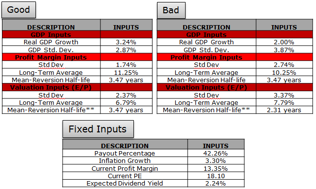
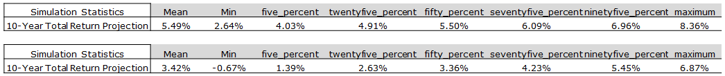
In the table below we have the summary statistics for the various inputs to give context as to the sanity of our model inputs.
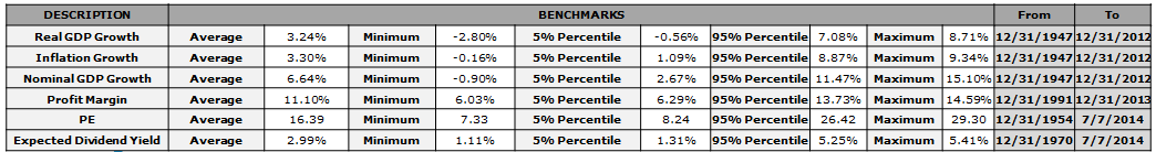
Click to enlarge. The results are hypothetical results and are NOT an indicator of future results and do NOT represent returns that any investor actually attained. Indexes are unmanaged, do not reflect management or trading fees, and one cannot invest directly in an index. Additional information regarding the construction of these results is available upon request.
What Does the Expected Returns Forecasting Model Spit out?
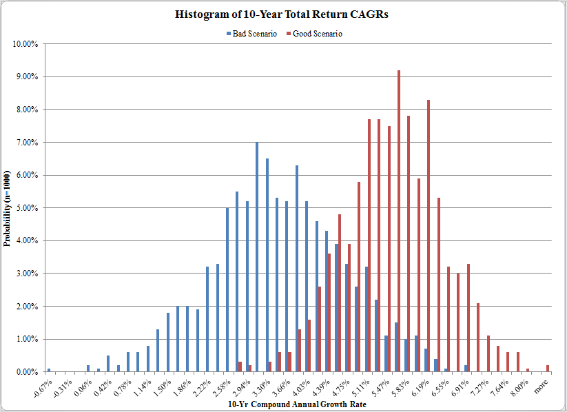
To generate these figures and the associated statistics below, we run 1,000 simulations of revenue growth, profit margins, and valuations and generate 1,000 possible 10-year total return estimates. We then plot them in the histogram below to show what is possible, given the model inputs outlined above.
The results are hypothetical results and are NOT an indicator of future results and do NOT represent returns that any investor actually attained. Indexes are unmanaged, do not reflect management or trading fees, and one cannot invest directly in an index. Additional information regarding the construction of these results is available upon request.
The figure above highlights the histogram of possible 10-Year total returns under the “good” and “bad” regimes discussed on the previous slide.
Under “good” conditions one can expect to earn 5.49% nominal CAGR over the next 10 years. With “bad” conditions, the expected CAGR drops to 3.42% and the distribution of CAGRs increases.
The results are hypothetical results and are NOT an indicator of future results and do NOT represent returns that any investor actually attained. Indexes are unmanaged, do not reflect management or trading fees, and one cannot invest directly in an index. Additional information regarding the construction of these results is available upon request.
What’s the Bottom Line on Return Forecasting?
The summary conclusion from all the return forecasting models–from the simple to the complex–is roughly the same. The complicated model we’ve described represents the “black box” sophisticated financial services firms and banks might peddle to the clients to justify ridiculous fees, but the reality is the silly simply Shiller Method will put you in the same ballpark. And the even more humbling reality is all of these models will almost certainly be wrong and generate nearly zero additional prediction ability over the long haul.
Moreover, even though we can build really cool models that “predict” the future, we don’t use them at all in our investment process. Why? Same reason we don’t deploy highly complex optimization models in our asset allocation systems: the estimation error of these return forecasting models is INSANE, and the signal/noise ratio is to high. So why bother adding complexity if it doesn’t add any value?
How’s that for inspiring news on the stock market expected returns prediction front?
References[+]
| ↑1 | Disclaimer: We recommend a realistic perspective on the viability of trying to predict market returns with quantitative models (we’ve written off the ability of “gut instinct” to forecast the future). The same holds for the complex model we outline below: 99% chance it doesn’t work any better than predicting the future based on astrology. |
|---|
About the Author: Wesley Gray, PhD
—
Important Disclosures
For informational and educational purposes only and should not be construed as specific investment, accounting, legal, or tax advice. Certain information is deemed to be reliable, but its accuracy and completeness cannot be guaranteed. Third party information may become outdated or otherwise superseded without notice. Neither the Securities and Exchange Commission (SEC) nor any other federal or state agency has approved, determined the accuracy, or confirmed the adequacy of this article.
The views and opinions expressed herein are those of the author and do not necessarily reflect the views of Alpha Architect, its affiliates or its employees. Our full disclosures are available here. Definitions of common statistics used in our analysis are available here (towards the bottom).
Join thousands of other readers and subscribe to our blog.