Executive Summary
In this article, we identify how we can improve the performance of the F-Score and enhance a generic value investing approach.
In a 2000 study, “Value Investing: The Use of Historical Financial Statement Information to Separate Winners from Losers” (Journal of Accounting Research, 2000), Joseph Piotroski examined whether an investor could improve his or her investment returns by using simple accounting-based fundamental analysis.
The F-Score is designed to identify fundamentally strong stocks within the cheapest stocks in the universe. For Piotroski, a cheap stock, or “value stock,” is defined as a stock with a high book value relative to its market price (in other words, a low price-to-book ratio). Professor Piotroski was inspired to find a better way to invest in value stocks, as a majority of value stocks (approximately 57%) underperform the market over one- and two-year stretches. Piotroski found that by identifying financially strong value stocks according to his F-Score, he could improve the return of a low price-to-book portfolio by at least 7.5% per year. In addition, he found that an investment strategy that bought expected winners and sold short expected losers generated a 23% annual return between 1976 and 1996.
Assuming that the “average [value stock] is financially distressed,” Piotroski chose nine fundamental signals to measure three areas of the stock’s financial health: profitability, financial leverage/liquidity, and operating efficiency. He sought to classify each fundamental signal into mutually exclusive states, as either “good” or “bad,” depending on the signal’s implication for a stock’s future prices and profitability. Each fundamental signal analyzed is expressed as a binary outcome. In other words, if the fundamental signal analyzed is good, it is marked as a one, and if the fundamental signal analyzed is bad, it is marked as a zero. The aggregate of the signals is the F-Score, which represents the sum of the nine binary signals. The aggregate signal is designed to measure the overall quality, or strength, of the stock’s financial health, and the decision to include the stock in a portfolio is ultimately based on the strength of the aggregate signal.
Analyzing the F-Score
Piotroski’s nine fundamental signals measure three areas of financial health: profitability; leverage, liquidity and source of funds; and operating efficiency.
Profitability
Piotroski uses four variables to measure a stock’s current profitability and cash flow realizations to glean information about the stock’s ability to generate funds internally. These performance-related variables are return on assets (ROA), cash flow from operations (CFO), the change in return on assets (ΔROA), and accruals (ACCRUAL). (Note that the Δ symbol refers to delta and means change in or difference, so ΔROA means change in ROA).
ROA and CFO are net income before extraordinary items and cash flow from operations, respectively, divided by beginning of the year total assets. If the stock’s ROA or CFO is positive, Piotroski defines the variable F_ROA or F_CFO as one, and zero if otherwise.
He defines ΔROA as the current year’s ROA less the prior year’s ROA. We are measuring not the static change in this profitability metric, but instead are scaling dynamically, using the firm’s asset base, which changes over time. If ΔROA is greater than 0, the variable F_ΔROA is marked one, and zero otherwise.
Piotroski defines the variable ACCRUAL as the stock’s current year’s net income before extraordinary items less cash flow from operations, scaled by beginning of the year total assets. The use of non-cash accruals is a signal that can contain information about the composition and quality of a firm’s earnings. The variable F_ ACCRUAL is marked one if CFO is greater than ROA, and zero if otherwise.
Leverage, Liquidity and Source of Funds
Piotroski’s F-Score assumes that an increase in leverage, deterioration in liquidity, or the use of external financing is an unfavorable signal about financial health. Three of the nine financial signals are therefore designed to measure changes in capital structure and the stock’s ability to meet future debt service obligations: ΔLEVER, ΔLIQUID, and EQ_OFFER.
ΔLEVER seeks to capture changes in the stock’s long-term debt levels. Piotroski measures ΔLEVER as the historical change in the ratio of total long-term debt to average total assets; he views an increase in financial leverage as a negative signal, and vice versa. By raising external capital, a financially distressed stock is signaling its inability to generate sufficient internal funds. In addition, an increase in long-term debt, relative to assets, is likely to place additional constraints on the stock’s financial flexibility. Piotroski marks the variable F_ΔLEVER as one if the stock’s leverage ratio fell in the preceding year, and zero if otherwise.
ΔLIQUID seeks to measure the historical change in the stock’s current ratio between the prior and current year, where Piotroski defines the current ratio as the ratio of current assets to current liabilities at fiscal year-end. Thus, has the firm’s current ratio increased or decreased, versus a year ago? He assumes that an improvement in liquidity is a good signal about the stock’s ability to service current debt obligations. The variable F_ΔLIQUID is marked one if the stock’s liquidity improved (increase in current ratio), and zero if otherwise.
F_EQISS measures whether a firm issued equity in the preceding year. The fact that these stocks are willing to issue equity when their stock prices are depressed highlights their poor financial health. F_EQISS captures whether a stock has issued equity in the year preceding portfolio formation. The variable F_EQISS is set to one if the stock did not issue common equity in the preceding year, and zero if otherwise.
Operating Efficiency
Piotroski’s two remaining signals—ΔMARGIN and ΔTURN—seek to measure changes in the efficiency of the stock’s operations and use of its assets. Piotroski believes these ratios are important because they reflect two key parts of the return on assets.
Piotroski defines ΔMARGIN as the stock’s current gross margin ratio (gross margin divided by total sales) less the prior year’s gross margin ratio. Piotroski believes that an improvement in margins signifies a potential improvement in costs, a reduction in inventory costs, or a rise in the price of the stock’s product, all of which are positive for the stock. The indicator variable F_ΔMARGIN equals one if ΔMARGIN is positive, and zero if otherwise.
Piotroski defines ΔTURN as the stock’s current year asset turnover ratio (total sales scaled by beginning of the year total assets) less the prior year’s asset turnover ratio. He says that an improvement in asset turnover signifies greater productivity from the asset base. Such an improvement can arise from more efficient operations (fewer assets generating the same levels of sales) or an increase in sales (which could also signify improved market conditions for the stock’s products). The indicator variable F_ΔTURN equals one if ΔTURN is positive, and zero if otherwise.
Now that we’ve defined all of the signals in the F-Score, let’s see how Piotroski combined them to find the F-Score, and then learn how to interpret the output.
F-Score Formula and Interpretation
Piotroski calculates his F-Score by summing the individual binary signals, or, more formally:
- F-Score = F_ROA + F_ΔROA + F_CFO + F_ ACCRUAL + F_ΔMARGIN + F_ΔTURN + F_ΔLEVER + F_ΔLIQUID + F_EQISS
An F-Score ranges from a low of zero to a high of nine, where a low F-Score represents a stock with very few good signals, and a high score indicates a stock with very many good signals. To the extent current fundamentals predict future fundamentals, the F-Score should indicate future stock returns. Piotroski’s investment strategy is simply to select value stocks with high F-Score signals.
Piotroski found that high F-Score value stocks beat the market by 13.4% per year versus 5.9% for the entire value quintile. This means that the high F-Score value stocks beat the average value stock by 7.5% per year (13.4% less 5.9%). The high F-Score value portfolio also contains a higher proportion of winners than the average portfolio. The high F-Score value portfolio picks winners 50% of the time. Clearly the F-Score discriminates between eventual winners and losers.
Piotroski’s F-Score is thus a useful and intuitive metric for value investors. His key insight is that quantitatively analyzing financial statements can improve performance. The F-Score is designed to eliminate underperforming stocks. It succeeds in doing so by classifying the stocks according to their financial health. The resulting returns to cheap, financially strong stocks are outstanding, albeit limited to stocks with small and medium market capitalization. In the next section, we discuss some small improvements to the F-Score that we use to enhance the ability of the financial statement analysis to separate the winners and losers.
Creating a Better F-Score
Piotroski’s F-score approach to identifying winners and losers is a good first step, but the F-score measure is, in the words of the author, ad hoc. Nobody wants their investment process to be ad hoc, but we do like the simplicity associated with the F-Score. In this section we do not intend to reinvent the wheel. Instead, we look to make intelligent changes to the F-Score that improve performance.
Using the F-Score as a foundation, we have created a new financial strength score (FS-Score), which we divide into the same three categories as the F-Score:
- Current profitability,
- Stability, and
- Recent operational improvements.
Like the F-Score, the FS-Score seeks to find the financially strongest stocks. We have modified the F-Score to tweak three variables and moved the variables into slightly more intuitive categories. The variables in our FS-Score are set out in the following manner.
Current Profitability
We use three variables to measure a stock’s current profitability and cash flow realization:
ROA and FCFTA are net income before extraordinary items and free cash flow, respectively, divided by most recent total assets. If the stock’s ROA or FCFTA is positive, we define the respective variable FS_ROA or FS_FCFTA as one, and zero if otherwise.
ACCRUAL is the stock’s current year’s net income before extraordinary items less cash flow from operations, scaled by beginning of the year total assets. The variable FS_ACCRUAL is marked one if FCFTA is greater than ROA, and zero if otherwise.
Our current profitability variables are similar to Piotroski’s profitability variables, except that we replace the CFO variable with free cash flow divided by total assets (FCFTA). We make this change to take into account the impact of capital expenditures on the stock’s cash flows. We also exclude the variable ΔROA from this category and put it and ΔFCFTA in our “recent operational improvements” category because we believe it is a more intuitive category for these variables.
Stability
Like Piotroski, we assume that an increase in leverage, deterioration in liquidity, or the use of external financing is a bad signal about financial health. Our stability signals measure changes in capital structure and the stock’s ability to meet future debt service obligations:
- ΔLEVER is the historical change in the ratio of total long-term debt to total assets. FS_ΔLEVER is marked one if the stock’s leverage ratio fell in the preceding year, and zero if otherwise.
- ΔLIQUID is defined as the year-over-year change in the ratio of current assets to current liabilities. The variable FS_ΔLIQUID is marked one if the stock’s liquidity improved (higher ratio), and zero if otherwise.
- NEQISS is equity repurchases minus equity issuance, or net equity issuance. FS_NEQISS is set to one if repurchases exceed equity issuance, and zero otherwise.
Our stability category differs from Piotroski’s in one important way: We replace the F-Score’s equity issuance variable, EQISS, with net equity issuance, or NEQISS, which is defined as repurchases minus issuances. We make this small, but important, change because we believe EQISS can be a misleading metric.
For example, many firms issue shares for a variety of reasons unrelated to financial health, including management or employee incentive programs. A company may issue a small number of shares to compensate a CEO, but simultaneously initiate a substantial repurchase program that dwarfs the number of shares issued to the CEO. Piotroski’s EQISS would penalize this stock because of the small equity issuance, while NEQISS would consider the relative size of both the buyback and the issuance and score accordingly. In this example, each metric would be scored in the following way: EQISS would be zero and have no effect on F-Score; NEQISS would increase by one and increase FS-Score.
(Note: We calculate NEQISS using the technique used in the August 2004 NBER working paper “On the Importance of Measuring Payout Yield: Implications for Asset Pricing,” by Jacob Boudoukh, Roni Michaely, Matthew Richardson and Michael Roberts.)
Recent Operational Improvements
We introduce a new section for the FS-Score: recent operational improvements. This category is roughly equivalent to the F-Score’s operating efficiency section, except that the focus in our FS-Score is on improvements. We include in our recent operational improvements category the following:
- ΔROA is the current year’s ROA less the prior year’s ROA. If ΔROA is greater than 0, the variable FS_ΔROA scores a one, and zero otherwise.
- ΔFCFTA is the current year’s FCFTA less the prior year’s FCFTA. If ΔFCFTA is greater than 0, the variable FS_ΔFCFTA is marked one, and zero otherwise.
- ΔMARGIN is the stock’s current gross margin ratio (gross margin divided by total sales) less the prior year’s gross margin ratio. The indicator variable FS_ΔMARGIN equals one if ΔMARGIN is positive, and zero if otherwise.
- ΔTURN is the stock’s current year asset turnover ratio (total sales scaled by beginning of the year total assets) less the prior year’s asset turnover ratio. The indicator variable FS_ΔTURN equals one if ΔTURN is positive, and zero if otherwise.
We examine recent operational improvements to ascertain whether the business has operational momentum. We don’t want to buy a seemingly cheap stock that gets increasingly expensive relative to its fundamentals because the business deteriorates. For example, a stock with $100 million in EBIT (earnings before interest and taxes) trading at a market value of $300 million is trading at a 3x multiple. If operations deteriorate to the extent that next year’s EBIT is only $50 million, the “bargain” price-to-EBIT ratio of 3.0 becomes a more expensive ratio of 6.0. If this halving of EBIT continues, we will be left holding a very expensive stock after a few years.
Does the Improved F-Score Work?
Our FS-Score has 10 metrics, versus Piotroski’s nine, across the three categories of profitability, stability, and recent operational improvements. The final score is from zero to 10, where 10 is a perfect score, and zero is the worst score possible. The FS-Score formula is as follows:
- FS-Score = FS_ROA + FS_FCFTA + FS_ACCRUAL + FS_ΔLEVER + FS_ΔLIQUID+FS_NEQISS + FS_ΔROA + FS_ΔFCFTA + FS_ΔMARGIN + FS_ΔTURN
To compare the performance of the F-Score and the FS-Score, we looked at the returns from all stocks with an F-Score of 6, 7, 8, or 9 and compared those to the performance of all FS-Scores with a score of 7, 8, 9, or 10. We examined the returns to a portfolio containing the high scorers in each strategy over the period from January 1, 1974, to December 31, 2014. Results are gross of management fee and transaction costs for illustrative purposes only. These are simulated performance results and do not reflect the returns an investor would actually achieve. All returns are total returns and include the reinvestment of distributions (e.g., dividends). Data is from Bloomberg, CRSP, and Compustat. Portfolios were rebalanced annually and we only examined firms above the New York Stock Exchange 40th percentile for market cap (currently around $1.8 billion) to avoid peculiar empirical effects associated with micro- and small-cap stocks. The results are shown in Table 1 and Figure 1.
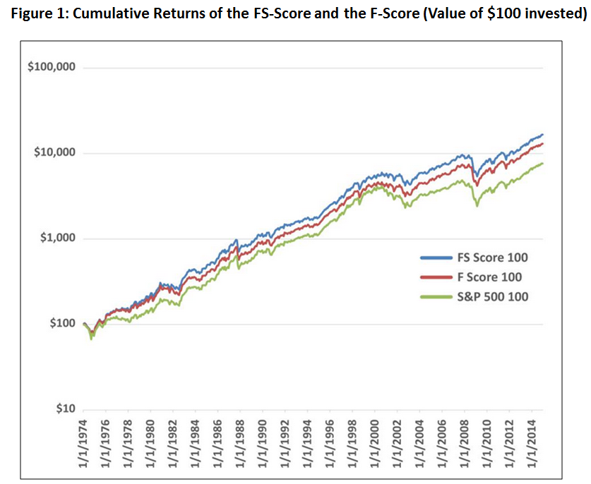
The results are hypothetical results and are NOT an indicator of future results and do NOT represent returns that any investor actually attained. Indexes are unmanaged, do not reflect management or trading fees, and one cannot invest directly in an index. Additional information regarding the construction of these results is available upon request.
Table 1. F-Score and FS-Score Performance (1974 to 2014)
| FS-Score | F-Score | S&P 500 | |
| Compound annual growth rate (%) | 13.3 | 12.6 | 11.2 |
| Standard deviation (%) | 15.2 | 15.3 | 15.5 |
| Downside deviation (%) | 10.7 | 10.9 | 11.1 |
| Sharpe ratio | 0.58 | 0.54 | 0.45 |
| Sortino ratio (min. accepted ret. = 5%) | 0.82 | 0.75 | 0.62 |
The results are hypothetical results and are NOT an indicator of future results and do NOT represent returns that any investor actually attained. Indexes are unmanaged, do not reflect management or trading fees, and one cannot invest directly in an index. Additional information regarding the construction of these results is available upon request.
The small tweaks we applied to the F-Score caused the FS-Score to outperform by a small but economically meaningful amount. Additionally, the structure of the FS-Score is more intuitive and grounded in value-investing philosophy than the F-Score.
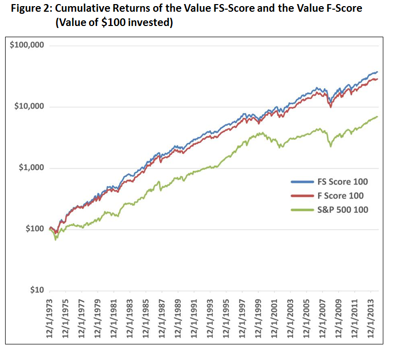
Next, we analyzed the F-Score and the FS-Score in the context of cheap stocks, which is more akin to the original study conducted by Piotroski. We looked at the returns from cheap stocks (defined as being in the 20% cheapest based on book-to-market, which is the inverse ratio of price-to-book) with an F-Score of 6, 7, 8, or 9 and compared those to the performance of cheap stocks with an FS-Score of 7, 8, 9, or 10. We examined the returns to the value portfolios containing the high scorers in each strategy over the period from January 1, 1974, to December 31, 2014, as shown in Table 2 and Figure 2.
The results are hypothetical results and are NOT an indicator of future results and do NOT represent returns that any investor actually attained. Indexes are unmanaged, do not reflect management or trading fees, and one cannot invest directly in an index. Additional information regarding the construction of these results is available upon request.
Table 2. Value Stocks and F-Score and FS-Score Performance (1974 to 2014)
| FS-Score | F-Score | S&P 500 | |
| Compound annual growth rate (%) | 15.9 | 15.2 | 11.2 |
| Standard deviation (%) | 15.4 | 15.2 | 15.5 |
| Downside deviation (%) | 10.2 | 10.4 | 11.1 |
| Sharpe ratio | 0.72 | 0.69 | 0.45 |
| Sortino ratio (min. accepted ret. = 5%) | 1.08 | 0.99 | 0.62 |
The results are hypothetical results and are NOT an indicator of future results and do NOT represent returns that any investor actually attained. Indexes are unmanaged, do not reflect management or trading fees, and one cannot invest directly in an index. Additional information regarding the construction of these results is available upon request.
Conclusion
We have identified ways to improve the baseline Piotroski F-Score and enhance value investing strategies. The final product is the FS-Score, which incorporates net-share repurchases and free-cash-flow metrics and arranges the metrics to align closer with traditional value-investing principles.
There are more sophisticated ways to create systematic value investing strategies, which we discuss in my co-authored book, “Quantitative Value” (John Wiley & Sons, 2012), from which this article was adapted. In the end, the evidence suggests that the most effective way to value invest is straightforward: Buy the cheapest, highest-quality value stocks.
About the Author: Wesley Gray, PhD
—
Important Disclosures
For informational and educational purposes only and should not be construed as specific investment, accounting, legal, or tax advice. Certain information is deemed to be reliable, but its accuracy and completeness cannot be guaranteed. Third party information may become outdated or otherwise superseded without notice. Neither the Securities and Exchange Commission (SEC) nor any other federal or state agency has approved, determined the accuracy, or confirmed the adequacy of this article.
The views and opinions expressed herein are those of the author and do not necessarily reflect the views of Alpha Architect, its affiliates or its employees. Our full disclosures are available here. Definitions of common statistics used in our analysis are available here (towards the bottom).
Join thousands of other readers and subscribe to our blog.