Tactical Asset Allocation: A Practitioner’s Defense of Return Predictability

The prospect of being able to successfully anticipate and predict future market returns is irresistible to practitioners and academics alike, although success has proven elusive. Many have fallen short while seeking this “holy grail” of investing.

For instance, Goyal and Welch (2008) examined fourteen different return forecasting variables, and concluded that these market-timing signals are unstable, and that as of 2005 most models had lost statistical significance. Estrada (2015) showed that tactical asset allocation rules using dividend yield, P/E and CAPE were useless in the short run, and that investors would be better off sticking with a simple 60/40 stock-bond portfolio. As National Medal of Science winner Robert Merton put it in a seminal 1980 paper, which was the first to anticipate a time-varying equity premium:

…if the expected return on the market were known to be a constant for all time, it would take a very long history of returns to obtain an accurate estimate. And, of course, if this expected return is believed to be changing through time, then estimating these changes is still more difficult…one might say that to attempt to estimate the expected return on the market is to embark on a fool’s errand.

Wow, that’s depressing rhetoric. So is market timing hopeless?

Perhaps not! Hope springs eternal. In a tribute to the indomitable human spirit and the insatiable curiosity of academics, researchers have continued to seek the holy grail of return predictability. Among the latest offerings from academia is a recent paper, “A Practitioner’s Defense of Return Predictability,” by Hull and Qiao, in which the authors present a model that seems to significantly enhance a simple buy-and-hold strategy. (Note: We have our own take here with regard to market timing and our classic “beware of geeks bearing formulas” piece).

Utilizing an Aggregate of Many Predictors

While there have been many branches within the predictability literature, studies have tended to focus on individual candidate variables, against which univariate regressions are run. The authors suggest that using a number of different variables may provide a broader information set, and disparate information about future returns, and at different time horizons. Hence, by combining them, they might jointly allow a superior return forecast. Of course, we must be very wary of data-mining when we go down this road. See here and here for some example research on this topic.

What is interesting about this paper?

• It uses a relatively large set of predictors (20 variables including technical indicators, macroeconomic variables, return based predictors, price ratios, commodity prices, etc.)
  • Previous literature: used a small set of predictors. Others have examined the joint forecasting power of predictors, such as Rapach, Strauss, and Zhou (2010), but these have tended to use smaller samples.
• It forecasts medium-term market returns (next six months).
  • Previous literature: Focused on predicting returns over 1) the long-term (one or more years) or 2) the very short-term (i.e., daily or weekly frequency) which tend to contain much more noise and where statistical evidence is more difficult to establish
• It uses correlation screening to filter out the least significant variables and combine the predictors.
  • Previous literature: often relied exclusively on ordinary least squares in forecasting regressions.
• Offers other new insights:
  • It combines predictors that forecast different horizon returns rather than those that forecast the same horizon.
  • It tries to eliminate look-ahead bias by including variables only after they have been discovered.
  • Looks at a trading strategy, and considers transaction costs and taxes

Below are the forecasting variables, which involve technical indicators, macroeconomic variables, returns based predictors, price ratios and others, which are combined using correlation screening.

20 Return Predictors:

1. Dividend-Price Ratio (DP); if dividend-price ratio is high, returns are likely to be high
2. Price-to-Earnings Ratio (PE); a high P/E indicates a low equity premium
3. Book-to-Market Ratio (BM); high book-to-market for S&P indicates high future returns
4. Cyclically Adjusted Price to Earnings Ratio (CAPE); the Shiller PE
5. Principal Component of Price Ratios (PCA-price); chooses largest principal component of DP, PE, BM and CAPE
6. Bond Yield (BY); moving average of 10-year bond yields
7. Default Spread (DEF); when Baa versus Aaa spreads are high, future returns are high.
8. Term Spread (TERM); Aaa bond versus 1-month treasury spread; again, high spreads = high returns
9. Cointegrating Residual of Consumption, Assets, and Wealth (CAY); these correlate with discount rates
10. Sell in May and Go Away (SIM); buys during November to April, sells during May to October.
11. Variance Risk Premium (VRP); VIX minus GARCH-style model
12. Implied Correlation (IC); high correlation of equity options leads to high future returns
13. Baltic Dry Index (BDI); 3-month change in BDI predicts intermediate global stock returns
14. New Orders/Shipments (NOS); new orders divided by shipments
15. Consumer Price Index (CPI); CP measure inflation, which explains 80% of mispricing
16. Ratio of Stock Price to Commodity Price (PCR)‘ ; uses log of ratio of SPY to GSCI
17. Moving Average (MA); simple 10-month moving average
18. Principal Component of Technical Indicators (PCA-tech); technicals used to identify business cycle peaks and troughs
19. Oil Price Shocks (OIL); Use oil term structure; if oil price changes are high, returns are low
20. Short Interest (SI); high short interest indicates low equity premium

A lot of this data can be found at Amit Goyal’s website: http://www.hec.unil.ch/agoyal/docs/PredictorData2015.xlsx.

Also, the authors present a document on how to replicate the results presented.

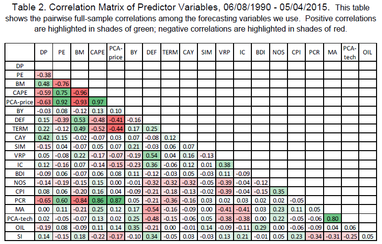
How Are These Variables Correlated?

The table below shows the pairwise correlations of these 20 forecasting variables (green is positive, red is negative).

The results are hypothetical results and are NOT an indicator of future results and do NOT represent returns that any investor actually attained. Indexes are unmanaged, do not reflect management or trading fees, and one cannot invest directly in an index. Additional information regarding the construction of these results is available upon request.

The good news is that these variables look to be different and the information carried by some signals has low correlation with the others. The bad news is that this estimation period is relatively short (~25 years) and correlation matrices are notoriously difficult to estimate with any degree of precision. So there is a non-trivial risk of a garbage in = garbage out type of problem.

Forecasting Results

Using daily data from 06/08/1990 through 05/04/2015, the paper runs three models: the first one is the “kitchen sink model,” which uses all 20 variables (hence the “kitchen sink”) all the time; the second one is the “correlation screening model“, which uses correlation screening in selecting individual forecasting variables; the third one is a “real-time correlation screening model,” which excludes look-ahead bias by including variables only after the time when they were discovered during the test.

• Correlation Screening: Using a look-back period of 10 years, only keep those variables that have at least 10% correlation with the upcoming 130-day returns.
• Real time: Use only variables that are known at the time. For example, OIL was first mentioned as a return predictor in 2005, so the model won’t include the OIL variable until 2005.

The graph below shows the variable selection for the “real-time correlation screening model.” The top figure shows the number of variables that are chosen in the model at any give time, and the bottom figure shows which variables are selected.

The results are hypothetical results and are NOT an indicator of future results and do NOT represent returns that any investor actually attained. Indexes are unmanaged, do not reflect management or trading fees, and one cannot invest directly in an index. Additional information regarding the construction of these results is available upon request.

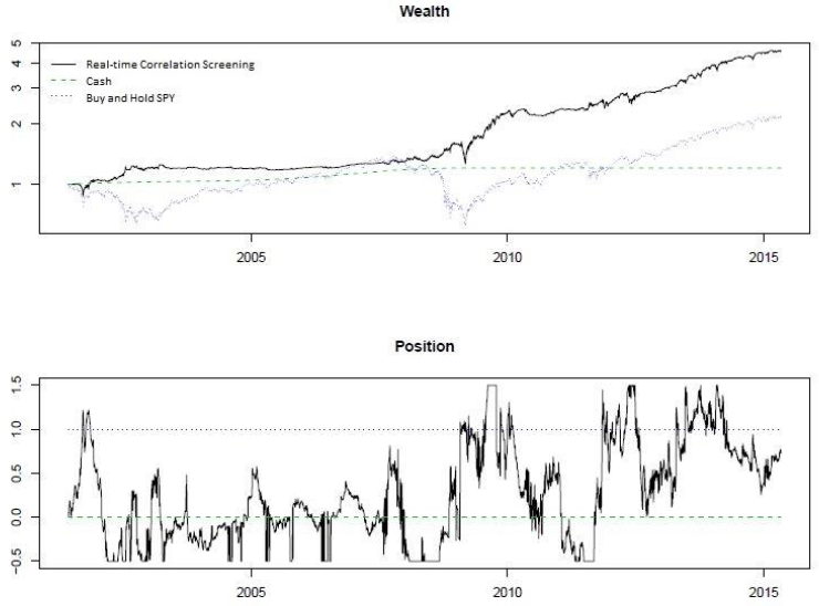
Every 20 days, the paper uses data from the previous 10 years to estimate model coefficients, and fixes the parameters for the next 20 days, at which time the model is run again. A simple strategy is to invest in two assets: SPY and cash. Everyday, we take positions in SPY based on the expected market return forecasts.

The below figure shows wealth accumulation using the strategy. We can see the obvious outperformance of the “real-time correlation screening model” against cash and simple buy-and-hold of SPY. During 2002 and 2008, this market-timing strategy helped avoid large drawdowns. The bottom panel shows the changing positions of the strategy. It has a cap of 150% long and 50% short of SPY.

The results are hypothetical results and are NOT an indicator of future results and do NOT represent returns that any investor actually attained. Indexes are unmanaged, do not reflect management or trading fees, and one cannot invest directly in an index. Additional information regarding the construction of these results is available upon request.

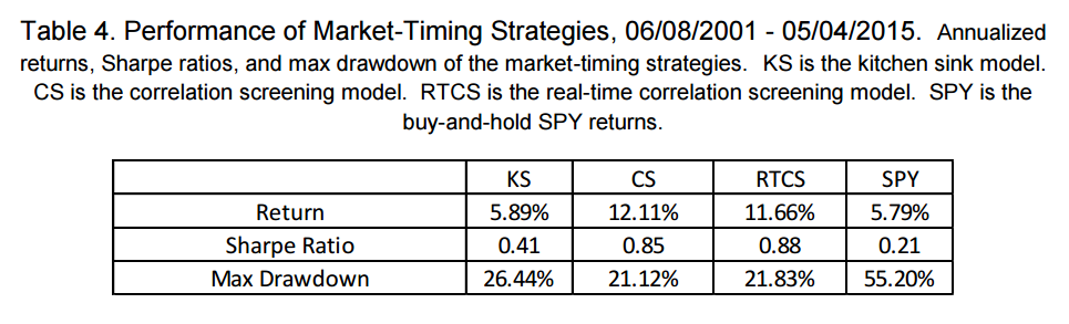
The paper also tests the economic magnitude of return predictability through simulation. From the paper:

“A simulation from June 8th 2001 through May 4th 2015 shows that taking daily positions in the SPDR S&P 500 ETF Trust (SPY) proportional to the estimated expected risk premium results in an annual return of over 12% with a Sharpe ratio of 0.85. The annual return is more than twice that of the buy-and-hold strategy, with a Sharpe ratio four times as high in the same period.”

The authors also highlight the performance of their models from June 2001 to May 2015:

The results are hypothetical results and are NOT an indicator of future results and do NOT represent returns that any investor actually attained. Indexes are unmanaged, do not reflect management or trading fees, and one cannot invest directly in an index. Additional information regarding the construction of these results is available upon request.

KS, CS, and RTCS are all models the authors find interesting and the overall author’s conclusion: not too shabby.

Can’t say I disagree that the results are impressive. The problem is that a simply 12 month trend-following applied to the S&P 500 over the same period has a Sharpe of .80 and amazing drawdown control!

One has to ask a basic question: Is all the complexity and the inclusion of additional variables worth the potential risks of overfitting and/or brain damage?

Time to be a Market Timer?

There are a lot of interesting ideas and themes running throughout this paper. For those who have buried themselves in the market timing literature, you are well aware that is can get overwhelming very quickly. This paper does a good job introducing the concept for practitioners and summarizing a lot of ideas that have been floated in stand-alone academic papers. Definitely worth a read for all investors.

As far as the effectiveness of market timing, we’ll leave readers with a quote from the paper:

As our understanding of return predictability changes, so will the stigma associated with market-timing strategies. Anybody who claimed to implement a “market-timing” strategy in the past 30 years would have been considered irresponsible; as such a strategy was thought to underperform the buy-and-hold strategy. In the upcoming 30 years, it is likely that it will be considered irresponsible to not engage in informed market-timing. Investors should change their asset allocation as estimates for expected returns change, in order to maximize the long-run growth rate of their investment.

We’ll also leave readers with a personal anecdote. We started a large consulting research project on tactical asset allocation in 2010 and concluded our research around 2012. We developed a process that was similar to the one described in this paper. Next, we started implementing the program. The strategy was fine in practice, but further robustness lead us to the conclusion there was a high probabililty of data-mining involved. We stopped running the program and moved on to simple trend-based systems, which work arguably as well as more complex systems, but don’t have the baggage associated with highly complex systems.

A Practitioner’s Defense of Return Predictability

• Hull and Qiao
• A version of the paper can be found here.
• Want a summary of academic papers with alpha? Check out our Academic Research Recap Category.

Abstract:

We revisit the issue of return predictability and show there is substantial predictive power in combining forecasting variables. Drawing from twenty variables that have been proposed in the return predictability literature, we use correlation screening to combine the variables and demonstrate forecasting power at the six-month horizon. We illustrate the economic significance of return predictability through a walk forward simulation in which positions in SPY are taken proportional to the model forecast equity risk premium. Our simulated strategy yields annual returns more than twice that of the buy-and-hold strategy, and a Sharpe ratio four times as large. To eliminate look-ahead bias, we further perform the simulation including variables as they are discovered in the literature, and find similar annual returns and Sharpe ratios. Although a market-timing strategy outperforms the market, it is difficult to implement. We include a detailed discussion on the various difficulties in implementing such a market-timing strategy.