In my previous blog post we considered the general weighted moving average. In this post we aim to give an overview of some specific types of moving averages. Specifically, we cover “ordinary” moving averages and mention some examples of exotic moving averages.
Ordinary Moving Averages
These are the most common types of moving averages used to time the market.(1)
Simple Moving Average
The Simple Moving Average (SMA) computes the arithmetic mean of n prices

In this moving average, each price observation has the same weight wi=1 (ψi = 1/n). The average lag time and smoothness of SMA are given by

Obviously, increasing the size of the averaging window increases both the smoothness and the average lag time of SMA.
Linear Moving Average
The SMA is, in fact, an equally-weighted moving average where an equal weight is given to each price observation. Many traders believe that the most recent stock prices contain more relevant information on the future direction of the stock price than earlier stock prices. Therefore, they argue, one should put more weight on the more recent price observations. To correct the weighting problem in the SMA, some traders employ the linearly weighted moving average.
A Linear (or linearly-weighted) Moving Average (LMA) is computed as

In the linearly weighted moving average the weights decrease in arithmetic progression. In particular, in LMA(n) the latest observation has weight n, the second latest n-1, etc. down to one.
The average lag time and smoothness of LMA are given by

For a sufficiently large size of the averaging window (when n≫1),

Therefore, for the same size of the averaging window, LMA has not only smaller lag time than that of SMA, but also lower smoothness.
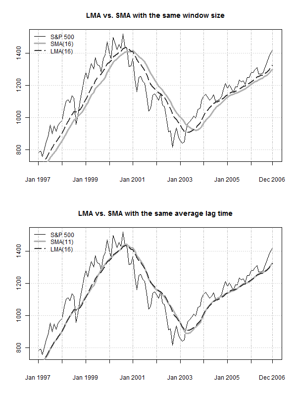
The figure below, top panel, demonstrates the values of SMA(16) and LMA(16) computed using the monthly closing prices of the S&P 500 index over a 10-year period from January 1997 to December 2006. This specific historical period is chosen for illustrations because over this period the trend in the S&P 500 index is clear-cut with two major turning points. Between the turning points, the index moves steadily upward or downward. Apparently, LMA(16) lags behind the S&P 500 index with a shorter delay than SMA(16). However, if traders want a moving average with a smaller lag time, instead of using LMA they can alternatively decrease the window size in SMA. Therefore, a fair comparison of the properties of the two moving averages requires using LMA and SMA with the same average lag time. The bottom panel in the figure below shows the values of SMA(11) and LMA(16) computed using the same stock index values.
Both moving averages have the same lag time of 5 (months). Rather surprisingly, contrary to the common belief that these two types of moving averages are inherently different, both of them move close together.
The results are hypothetical results and are NOT an indicator of future results and do NOT represent returns that any investor actually attained. Indexes are unmanaged, do not reflect management or trading fees, and one cannot invest directly in an index. Additional information regarding the construction of these results is available upon request.
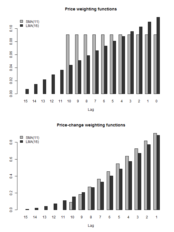
To illustrate the source of confusion and help explain why SMA and LMA with the same lag time are very similar, the next figure, top panel, plots the price weighting functions of SMA(11) and LMA(16). Obviously, the two price weighting functions are intrinsically different because seemingly each price lag contributes generally very differently to the value of a moving average. This gives rise to the belief that the values of these two moving averages differ a lot. In contrast, the bottom panel in the same figure plots the price-change weighting functions of SMA(11) and LMA(16), and both of these weighting functions look essentially similar. In particular, the differences in the two price-change weighting functions are marginal. This helps explain why the two moving averages move largely right together. Therefore it could be argued that a price-change weighting function provides a much more relevant information about the properties of a moving average than the corresponding price weighting function.
The results are hypothetical results and are NOT an indicator of future results and do NOT represent returns that any investor actually attained. Indexes are unmanaged, do not reflect management or trading fees, and one cannot invest directly in an index. Additional information regarding the construction of these results is available upon request.
Why the price-change weighting function is more relevant than the price weighting function in the analysis of properties of moving averages?
For the sake of illustration, let us consider a simple example of SMA(3) which is computed as

In this form, it looks like all prices are equally important. But, on the other hand, recall that

That is, the sequence of prices exhibits time-series dependency. For example, the price P2 consists of the sum of the previous price P1 and the price change ΔP1. Therefore the price P2 depends on the price P1. Put differently, the price P2 includes the price P1. Similarly, the price P3 depends on the price P2; the price P3 includes the price P2 which, in its turn, includes the price P1. In contrast, the sequence of price changes is close to be independent. Specifically, most of the time, ΔP2 is independent of ΔP1 etc.
The formula for SMA(3) can be presented in terms of price changes:

In words, the value of SMA(3) equals the first (last) closing price plus (minus) the linear moving average of the previous price changes. The moral is that focusing on the price weighting function creates an illusion that all price observations are equally important, but it is not true since price series exhibits strong serial dependency. In reality, what important is the changes between the successive observations (because they can be assumed to be independent) and the weighting of these changes.
Exponential Moving Average
A disadvantage of the linearly weighted moving average is that its weighting scheme is too rigid. This problem can be addressed by using the exponentially weighted moving average instead of the linearly weighted moving average. An Exponential Moving Average (EMA) is computed as

where 0<λ≤1 is a decay factor. When λ<1, the exponentially weighted moving average assigns greater weights to the most recent prices. By varying the value of λ, one is able to adjust the weighting to give greater or lesser weight to the most recent price.
The average lag time of EMA depends on the value of two parameters: the decay factor λ and the size of the averaging window n. For example, to reduce the average lag time, one can either reduce the window size n or decrease the decay factor λ. Consequently, there are infinitely many combinations of {λ,n} that result in EMAs with exactly the same lag time; at the same time these moving averages have similar type of the weighting function. As a result, these EMAs possess basically similar properties.
To get rid of the unwarranted redundancy in the parameters of the EMA with a finite size of the averaging window, traders use EMA with an infinite size of the averaging window. Specifically, traders compute EMA as

For an infinite EMA, the average lag time is given by

Even though an infinite EMA is free from the redundancy of a finite EMA, using EMA together with the other types of moving averages is inconvenient because the key parameter of EMA is the decay constant, whereas in both SMA and LMA the key parameter is the size of the averaging window. To unify the usage of all types of moving averages, traders also use the size of the averaging window as the key parameter in the (infinite) EMA. The idea is that EMA with the window size of n should have the same average lag time as SMA with the same window size. Equating the lag time of SMA(n) with the lag time of EMA(λ) gives

The solution of this equation with respect to λ yields

As a result, EMA is computed according to the following formula:

The smoothness of EMA equals

Therefore, not only the average lag time of EMA(n) equals the average lag time of SMA(n), but also the smoothness of both these moving averages is alike (at least in theory).
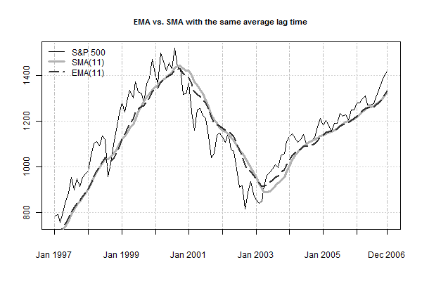
The figure below plots the values of SMA(11) and EMA(11) computed using the monthly closing prices of the S&P 500 index over a 10-year period from January 1997 to December 2006. Both of the moving averages have the same average lag time of 5 (months). The plot in this figure suggests that the values of SMA(11) and EMA(11) move close together when the stock prices trend upward or downward. This comes as no surprise given the previously established fact that all moving averages with different weighting functions but the same average lag time move close together when the trend is strong. Only when the direction of trend is changing, we see that the values of SMA(11) and EMA(11) start to move slightly apart. The plot in this figure motivates that when the direction of trend is changing, EMA follows the trend more closely and, thus, might have a potential advantage over SMA with the same average lag time.
The results are hypothetical results and are NOT an indicator of future results and do NOT represent returns that any investor actually attained. Indexes are unmanaged, do not reflect management or trading fees, and one cannot invest directly in an index. Additional information regarding the construction of these results is available upon request.
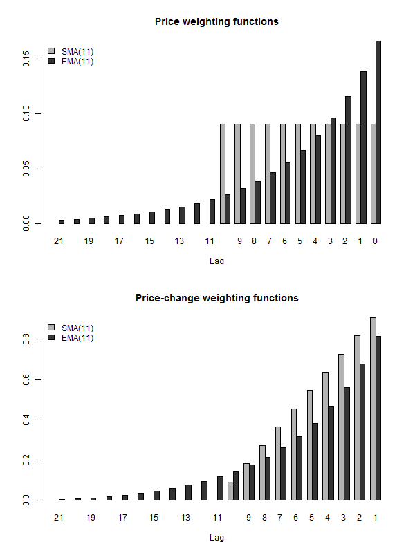
The next figure plots the price weighting functions (top panel) and the price-change weighting functions (bottom panel) of SMA(11) and EMA(11). For EMA, not only the price weighting function is substantially different from that of SMA, but there are also notable (yet not very significant) differences between the two price-change weighting functions.
The results are hypothetical results and are NOT an indicator of future results and do NOT represent returns that any investor actually attained. Indexes are unmanaged, do not reflect management or trading fees, and one cannot invest directly in an index. Additional information regarding the construction of these results is available upon request.
Even though SMA(n) and EMA(n) have the same smoothness and the same average lag time, EMA(n) follows the trend a bit more closely than SMA(n). To further highlight the difference between SMA and EMA with the same average lag time, we apply SMA(11) and EMA(11) to an artificial stock price trend. This artificial stock price trend is given by two linear segments. First, the stock price trends upward, then downward. Our goal is to visualize the behavior of SMA(11) and EMA(11) along the stock price trend in general, and their reactions to a sharp change in the trend in particular. The illustration is provided in the figure below. As expected, both moving averages generally move together; yet there are marginal but noticeable differences in the values of the two moving averages around their tops. Specifically, when the prices are trending, both of the moving averages lag behind the trend by 5 periods. However, while the turning point in SMA(11) lags behind the turning point in the trend by 5 periods, the turning point in EMA(11) lags behind the turning point in the trend by 3 periods (this delay time is computed numerically).
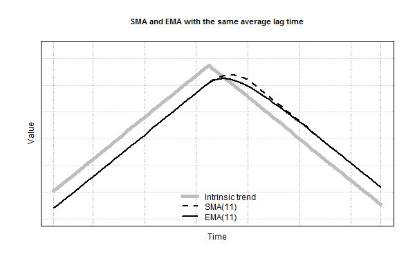
The results are hypothetical results and are NOT an indicator of future results and do NOT represent returns that any investor actually attained. Indexes are unmanaged, do not reflect management or trading fees, and one cannot invest directly in an index. Additional information regarding the construction of these results is available upon request.
The last illustration motivates us to draw the following conclusions:
- Moving averages that overweight the most recent prices may indeed possess an advantage over the equally-weighted moving average. This advantage consists in a bit earlier detection of turning points in a trend. Therefore in market timing applications both LMA and EMA might be superior to SMA. Yet, since the price is very noisy, this advantage might be completely nullified by noise.
- The quantity, known as the “average lag time” of a moving average, provides a correct numerical characterization of the time lag between the price and the value of the moving average only when prices are steadily increasing or decreasing. The “average lag time” has little to do with the delay in the identification of turning points in a trend.
Exotic Moving Averages
Besides the ordinary moving averages, there are exotic types of moving averages. These moving averages include moving averages of moving averages and moving averages with less lag time. In this blog post we only mention some of them.
Moving Averages of Moving Averages
Increasing the size of the averaging window is not the only way to improve smoothing properties of a moving average. Another possibility is to smooth a moving average by another moving average. The result of this operation is a new moving average which is usually called a “double moving average.” A double moving average can itself be smoothed further by another moving average producing a “triple moving average.” Such an iterative smoothing can be repeated a number of times, if desired. Some examples of this type of moving averages are as follows:
- Triangular moving average. It is a simple moving average of prices smoothed by another simple moving average with the same size of the averaging window. Therefore the triangular moving average can be denoted by SMASMA.
- Double exponential smoothing (EMAEMA). It is the recursive application of EMA two times.
- Triple exponential smoothing (EMAEMAEMA). It is the recursive application of EMA three times.
Moving Averages With Less Lag Time
The smoothness of a moving average is generally related to its lag time. That is, as a rule, the better the smoothness of a moving average is, the larger its lag time. There have been many attempts to improve the tradeoff between the smoothness and the lag time of a moving average. Examples of moving averages with less lag time are as follows:
- Zero Lag Exponential Moving Average (ZLEMA) by Ehlers and Way (2010);
- Double Exponential Moving Average (DEMA) by Mulloy (1994a);
- Triple Exponential Moving Average (TEMA) by Mulloy (1994b);
- Hull Moving Average (HMA) by Hull (2005).
The common feature of these moving averages is that the price weighting functions of these moving averages assign negative weights to more distant prices in the averaging window. For the sake of illustration, consider ZLEMA which is constructed on the basis of EMAs. The figure below plots the price weighting function of ZLEMA as well as the price weighting function of EMA(11) used to create this ZLEMA. Notice that in ZLEMA the weights of the price lags from 5 and beyond are negative.
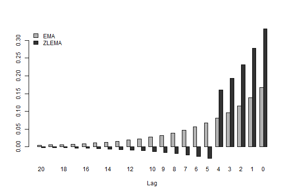
The results are hypothetical results and are NOT an indicator of future results and do NOT represent returns that any investor actually attained. Indexes are unmanaged, do not reflect management or trading fees, and one cannot invest directly in an index. Additional information regarding the construction of these results is available upon request.
Recall the formula for the computation of the average lag time of a moving average:

where ψi is the (normalized) price weighting function of a specific moving average. The average lag time is computed as the weighted average “age” of data used to compute the moving average of prices. If one allows negative weights in the price weighting function of a moving average, one can reduce the average lag time to zero. In principle, one can make the average lag time to be even negative. In this case it may seem that a moving average, instead of being a lagging indicator, becomes miraculously a leading indicator and can easily predict the turning points in the stock price trend. Unfortunately, miracles do not happen in the real world. In this context, it is worth repeating that only in cases where the prices are steadily increasing or decreasing, the “average lag time” provides a correct numerical characterization of the time lag between the price and the value of the moving average.
Despite the fact that these moving averages have almost zero average lag time, all of them identify turning points in a trend with delay. For the sake of illustration, the figure below shows the behavior of EMA and ZLEMA along the familiar artificial stock price trend. Notice that, when the prices are trending, ZLEMA follows the trend with almost zero lag. However, when the direction of the trend is sharply changing, ZLEMA needs time to adapt to the new direction of the trend. During this “adaptation period”, ZLEMA lags behind the trend. Consequently, this illustration demonstrates that ZLEMA has almost zero lag time only when prices are trending steadily over a relatively long period. Our analysis reveals that when both an ordinary moving average and a moving average with a less lag time have the same lag time in turning point identification, the ordinary moving average has better smoothness. Therefore in our opinion it is very unlikely that in market timing applications the moving averages with a less lag time are superior to the ordinary moving averages.
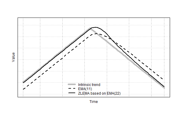
The results are hypothetical results and are NOT an indicator of future results and do NOT represent returns that any investor actually attained. Indexes are unmanaged, do not reflect management or trading fees, and one cannot invest directly in an index. Additional information regarding the construction of these results is available upon request.
Summary
We considered all ordinary moving averages used by traders and a few exotic moving averages. The exotic moving averages include moving averages of moving averages and mixed moving averages with less lag time. Each of these moving averages (both ordinary and exotic) has a unique weighting function and, therefore, each of these moving averages generally provides different tradeoff between the lag time and smoothness.
The fallacy that is usually committed by traders is to think that one can deduce the properties of a moving average by looking at the shape of its price weighting function. For example, the common belief is that LMA (or EMA) is very much different from SMA. By means of illustrations, we demonstrated that the properties of a moving average are revealed not by its price weighting function, but by its price-change weighting function. The correct comparison of the properties of two different moving averages should be done by looking at their price-change weighting functions when the two moving averages have either the same average lag time or the same smoothness. Our analysis shows that, when two ordinary moving averages have the same average lag time, their price-change weighting functions differ marginally.
We assert that the notion of the “lag time” of a moving average is an elusive concept. Previously we argued that the quantity, known as the “average lag time” of a moving average, provides a correct numerical characterization of the time lag between the price and the value of a moving average of prices only when prices are steadily increasing or decreasing. Our analysis reveals that there are two issues with the notion of the “average lag time.” First, the average lag time has little to do with the delay in the identification of turning points in a trend. Second, the average lag time can be easily reduced (that is, manipulated) by using a weighting function with negative weights. However, this reduction in the average lag time does not translate into a reduction in the delay time in turning point identification.
Our analysis demonstrates that, as compared with equally-weighted moving average, ordinary moving averages that overweight the most recent prices provide a better tradeoff between the smoothness and the delay in turning point identification. This fact suggests that LMA and EMA might have some potential advantages over SMA in market timing applications. Our analysis also suggests that moving averages with reduced (by means of using negative weights in a weighting function) average lag time have worse tradeoff between the smoothness and the delay in turning point identification than that provided by the ordinary moving averages.
Additional Resources for Self-Study
The reader can study the properties of different moving averages using these interactive web illustrations. These illustrations allow one to select two moving averages and compare their weighting functions, their values computed using the closing prices of the S&P 500 stock price index, and their reactions to a sharp change in an artificial stock price trend.
References
Ehlers, J. F. and Way, R. (2010) “Zero Lag (Well, Almost)”, Technical Analysis of Stocks and Commodities, 28 (12), 30–35.
Hull, A. (2005). “How to Reduce Lag in a Moving Average“. [Online; accessed 7-October-2016] Mulloy, P. G. (1994a). “Smoothing Data With Faster Moving Averages”, Technical Analysis of Stocks and Commodities, 12 (1), 11–19.
Mulloy, P. G. (1994b). “Smoothing Data With Less Lag”, Technical Analysis of Stocks and Commodities, 12 (2), 72–80.
References[+]
| ↑1 | Alpha Architect uses this type of moving average in their trend-following systems. |
|---|
About the Author: Valeriy Zakamulin
—
Important Disclosures
For informational and educational purposes only and should not be construed as specific investment, accounting, legal, or tax advice. Certain information is deemed to be reliable, but its accuracy and completeness cannot be guaranteed. Third party information may become outdated or otherwise superseded without notice. Neither the Securities and Exchange Commission (SEC) nor any other federal or state agency has approved, determined the accuracy, or confirmed the adequacy of this article.
The views and opinions expressed herein are those of the author and do not necessarily reflect the views of Alpha Architect, its affiliates or its employees. Our full disclosures are available here. Definitions of common statistics used in our analysis are available here (towards the bottom).
Join thousands of other readers and subscribe to our blog.

