Trend-Following with Valeriy Zakamulin: Performance Measurement and Outperformance Tests (Part 5)

We consider an investor and a financial market that consists of only two assets: one risky asset and one safe (or risk-fee) asset. An example of a risky asset is an investable stock market index. When it comes to the safe asset, even though financial theory assumes its existence, there are no completely risk-free assets in financial markets. A short-term Treasury bill (with time to maturity from one to three months) commonly serves as a proxy for the risk-free asset. This is because these Treasury bills have virtually no default risk and their return is known in advance with rather high precision.

We suppose that the investor wants to invest for a long term and, therefore, one possibility is to buy and hold the risky asset. The other possibility is to implement a trend-following strategy which consists of switching between the risky asset and the risk-free asset. How to decide which strategy to prefer? Answering this question starts with obtaining historical returns to the risky asset, r_B, and the risk-free asset, r_f. Then the investor simulates the returns to the trend-following strategy, r_A. So far everything is easy and trivial. The next problem is crucial but much more difficult: by comparing the properties of the two return series, r_B and r_A (subscripts B and A denote the buy-and-hold strategy and the active strategy respectively), the investor needs to decide which strategy is better. Unfortunately, there is no unique solution to this paramount problem. The goal of this blog post is to describe the alternative solutions, their advantages and disadvantages, and practical complications.

Performance Measures

By a performance measure in finance one means a score attached to each risky asset. This score is usually used for the purpose of ranking of risky assets. That is, the higher the performance measure of an asset, the higher the rank of this asset. The asset with the highest rank is considered the best asset for investment. Therefore the goal of any investor who uses a particular performance measure is to select the asset for which this measure is the greatest.

At first sight it seems rather natural to use the mean (or expected) return as a performance measure. That is, denoting by E[.] the expectation operator, the investor compares E[r_B] and E[r_A] and selects the asset with the highest mean return. The problem with using the mean return as a performance measure is as follows. When the risk-free asset is present and there are no limitations on borrowing and lending at the risk-free rate, by using leverage the investor can attain any desirable level of mean return. In fact, the role of the risk-free asset is to control the risk of the investor’s portfolio. That is, the investor with a low risk tolerance can reduce the risk by investing only a fraction of his money into the risky asset and the rest into the risk-free asset. The investor with a high risk appetite can borrow money at the risk-free rate and invest all own money and the borrowed money into the risky asset.

Generally, the investor creates a portfolio by mixing a risky asset and the risk-free asset. As a result, the investor’s “capital allocation” consists of investing proportion a in the risky asset r_i (i∈{A,B}) and, consequently, 1-a in the risk-free asset. The return on the investor’s complete portfolio is given by

Notice that if 0<a<1, the investor splits his money between the risky and the risk-free asset. If a=1, the investor’s money is placed in the risky asset only. Finally, if a>1, the investor borrows money at the risk free rate and invests all own money and borrowed money in the risky asset. The expected return on the investor’s complete portfolio is given by

Observe that when E[r_i-r_f]>0 and borrowing at the risk-free interest rate is not limited, the investor can attain any level of expected return. Using the expected return as a performance measure is equivalent to assuming that the investor’s goal is to maximize the expected return on his complete portfolio. If the investor behaves as though his objective function is to maximize the expected return, such an investor would be willing to borrow an infinite amount at the risk-free rate and invest it in the risky asset. Thus, the expected return decision criterion produces a paradox. In particular, a seemingly sound criterion predicts a course of action that no actual investor would be willing to take.

The expected return of a risky asset, often termed as the “reward” measure, is an important measure that characterizes the properties of a risky asset. The other important characteristic of a risky asset is its measure of risk. The paradox presented above appears because we assume that in making financial decisions the investor ignores risk. When we assume that the goal of each investor is to choose a risky asset that provides the best tradeoff between the risk and reward, we arrive to a so-called “reward-to-risk” measure.

The best known reward-to-risk measure is the Sharpe ratio. In addition to the original Sharpe ratio, there are almost a hundred alternatives to the Sharpe ratio, see a review paper by Cogneau and Hubner (2009). Most of these alternatives are ad-hoc ratios of a measure of reward to a measure of risk. And most of these measures are not rational reward-to-risk measures. It is therefore instructive, by the example of the Sharpe ratio, to consider the justification of a rational reward-to-risk measure.

Modern financial theory suggests that the choice of the best risky asset depends on the investor’s risk preferences that are generally described by a utility function. In the mean-variance framework of Markowitz portfolio theory, the utility from the investor’s complete portfolio is given by

where E[r_Ci] and σ_Ci denote the mean and standard deviation of returns, respectively, of the investor’s complete portfolio created using asset i, and R is the investor’s risk aversion coefficient. In this framework, the standard deviation is a measure of risk. The coefficient 1/2 is chosen for the sake of convenience. Observe that the higher the expected return, the higher the utility. Conversely, the higher the risk, the lower the utility. The risk aversion coefficient is specific for each investor and measures the investor’s desirable tradeoff between the risk and reward. For example, it allows us to compute the reward the investor requires for taking some particular amount of risk.

The standard deviation of the investor’s complete portfolio (see equation 1) is given by

Therefore the utility from the investor’s complete portfolio can be re-written as

According to modern financial theory, the choice of the best risky asset is made as follows. First, the investor maximizes the utility from investing in the risky asset r_B. It is important to note that in order to do this, the investor needs to find the optimal proportion a, that is, to solve the following optimization problem:

Denote this maximum investor’s utility from investing in asset r_B by U*(r_CB). Second, the investor maximizes the utility from investing in the risky asset r_A; denote this utility by U*(r_CA). Finally, the investor compares U*(r_CB) and U*(r_CA) and selects the assets which provides the highest utility.

William Sharpe (see Sharpe, 1966, and Sharpe, 1994) was the first to observe that, in the mean-variance framework where investors can borrow and lend at the risk-free rate, the choice of the best risky asset does not depend on the investor’s attitude toward risk. Moreover, the choice of the best risky asset can be made without solving the two maximization problem. Sharpe’s approach is as follows. The combination of equations (2) and (3) yields the following relationship between the expected return and the risk of the complete portfolio:

Equation (4) says that there is a linear relation between the mean and standard deviation of returns of the investor’s complete portfolio. In the standard deviation – mean return space, this straight line is called the Capital Allocation Line (CAL). It depicts all risk-return combinations available to investors who allocate money between the risk-free asset and risky asset i. The intercept and the slope of the straight line equal r_f and E[r_i-r_f]/σ_i respectively. Sharpe showed that the asset with the highest slope of the capital allocation line should be preferred by all investors. Therefore the slope of the capital allocation line can be used to measure the performance of a risky asset. William Sharpe originally called this slope as “reward-to-variability” ratio. Later this ratio was termed the “Sharpe ratio”:

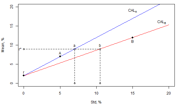
For the sake of illustration, the figure below indicates the locations of two risky assets, A and B, and the risk-free asset in the standard deviation – mean return space. Since the slope of the capital allocation line through A is higher than that through B, all investors prefer asset A to asset B. To realize this, suppose that the investor wants to attain some arbitrary level of mean returns r*. If the investor chooses asset A for capital allocation, the risk-return combination of the investor’s complete portfolio is given by point “a” that belongs to the capital allocation line through asset A. In contrast, if the investor chooses asset B for capital allocation, the risk-return combination of the investor’s complete portfolio is given by point “b” that belongs to the capital allocation line through asset B. Obviously, since both combinations, “a” and “b”, have the same mean return but “a” is less risky than “b”, any investor prefers “a” to “b”. Consequently, any investor chooses asset A.

The results are hypothetical results and are NOT an indicator of future results and do NOT represent returns that any investor actually attained. Indexes are unmanaged, do not reflect management or trading fees, and one cannot invest directly in an index. Additional information regarding the construction of these results is available upon request.

The Sharpe ratio is often criticized on the grounds that the standard deviation is not an adequate risk measure. In particular, the standard deviation penalizes similarly both the downside risk and upside return potential. Many researchers and practitioners argue that a proper risk measure must take into account only downside risk. They replace the standard deviation in the Sharpe ratio by an alternative risk measure ρ(r_i) and suggest a new alternative performance measure

However, the majority of the alternative risk measures are not rational because a rational risk measure must satisfy the following property (for a more detailed explanation, see Zakamulin, 2010):

The justification of this property is as follows. If a=0, then there should be no risk. When we begin to increase the value of a, the risk measure should be proportional to a, that is, proportional to the amount invested in the risky asset (in other words, twice the risk is twice as risky). A failure to satisfy this property means that a capital allocation line in the risk – mean return space is not a straight line and, as a result, the choice between two risky assets is no longer unique. A failure to satisfy this property also means that one can manipulate the value of a performance measure by changing the capital allocation (that is, the value of a).

However, a great deal of the alternative performance measures can be transformed to a correct rational form. Let us consider the Sortino ratio (see Sortino and Price, 1994) which is the most popular alternative to the Sharpe ratio. The original Sortino ratio is given by

where τ is the target or required rate of return for the investment strategy and θ_i is the target semi-deviation or downside variation computed as E[min(r_i-τ,0)²]. The advantage of the Sortino ratio is that the downside variation takes into account only the downside risk. The problem with the original Sortino ratio is that unless τ=r_f the capital allocation lines in the downside standard deviation – mean return space are not straight lines. The only rational form of the Sortino ratio is this one

Advantages and Disadvantages of all Performance Measures

The only advantage of any performance measure is that it allows the investor to make a simple and unique choice of the best risky asset regardless of the investor’s level of risk tolerance. But this advantage comes at the expense of making lots of necessary assumptions:

• All investors agree on the same performance measure. What if they do not? Different performance measures may produce different rankings of risky assets. As a result, the best risky asset according to one performance measure may be an inferior asset according to another performance measure.
• It is assumed that the borrowing at the risk-free rate is unlimited. In reality, borrowing at the risk-free rate is either restricted or just impossible. In this case the investor cannot attain any arbitrary level of mean returns. For example, in the illustration on the figure above the investor cannot attain r* using asset A in the capital allocation. As a consequence, risk tolerant investors tend to prefer asset B even though it has a lower Sharpe ratio;
• The assumption about the existence of a risk-free asset is very critical. Without the existence of a risk-free asset the choice of the best risky asset is generally not unique. The choice of the best risky asset is unique only in cases where, for example, E[r_A]>E[r_B] and at the same time ρ(r_A)<ρ(r_B); in this case asset A is better than asset B because asset A has greater expected return with lesser risk. In the other case where E[r_A]>E[r_B] and at the same time ρ(r_A)>ρ(r_B), asset A is more risky and more rewarding than asset B. In this case risk tolerant investors tend to choose asset A, whereas risk averse investors tend to prefer asset B;

The reader is reminded that, according to modern finance theory, the investor’s ultimate goal is not to maximize the Sharpe ratio (or any other performance measure) of his complete portfolio, but to maximize the utility that can be derived from this portfolio (for example, in terms of the final investor’s wealth). And in order to maximize the utility the investor has to solve two interrelated problems: (1) select the optimal risky asset and (2) select the optimal capital allocation between the risk-free asset and the (optimal) risky asset. The Sharpe ratio allows the investor to solve only one problem: to select the optimal risky asset. However, the ultimate investor’s goal is not fulfilled unless the investor selects the optimal capital allocation.

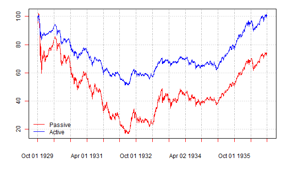
For the sake of illustration, the figure below plots the cumulative returns to two strategies over the period from October 1929 to September 1936. The cumulative return to the passive strategy is plotted in red color; the cumulative return to the active (volatility-responsive) strategy is plotted in blue color. The start date of the historical period coincides with the start of the stock market crash of October 1929 and the beginning of the Great Depression. By the end date of the historical period the cumulative return to the active strategy equals zero. Observe that by the end date the cumulative return to the passive strategy amounts to approximately -30%. This figure was shown to the students taking a postgraduate course on investments as well as to some of my academic colleagues. The following question was asked: which strategy would you prefer to invest to? All responses were unanimously in favor of the active strategy. And then they were told that the Sharpe ratio of the passive strategy is (slightly) above the Sharpe ratio of the active strategy and, therefore, by the Sharpe ratio criterion all rational investors (with mean-variance preferences) must prefer the passive strategy. Big surprise!

The results are hypothetical results and are NOT an indicator of future results and do NOT represent returns that any investor actually attained. Indexes are unmanaged, do not reflect management or trading fees, and one cannot invest directly in an index. Additional information regarding the construction of these results is available upon request.

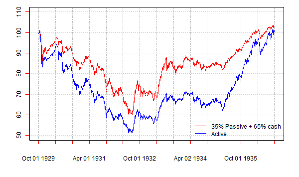
How come the investor should prefer the passive strategy that loses money over the given historical period? The resolution of this apparent paradox is as follows. The fact that the investor has to select the asset with the highest Sharpe ratio does not mean that the investor has to invest all money in this asset. The passive strategy is about 3 times as risky as the active one, judging by standard deviation. We can apply the same reasoning as that by William Sharpe. Suppose that the riskiness of the active strategy corresponds to the risk appetite of the investor. We can create another strategy with the same riskiness by investing 35% in the passive strategy and the rest, 65%, in the risk-free asset (that is, cash). The figure below plots the cumulative returns to the active strategy and the “adjusted” passive strategy. Now it becomes obvious that, given the fact that the two strategies are equally risky, the “adjusted” passive strategy provides higher return. The moral is that you cannot eat the Sharpe ratio. The Sharpe ratio facilitates the solution of the first problem: to select the best risky asset. But in order to take advantage of the best risky asset, the investor has to solve the second problem: to select the optimal capital allocation.

The results are hypothetical results and are NOT an indicator of future results and do NOT represent returns that any investor actually attained. Indexes are unmanaged, do not reflect management or trading fees, and one cannot invest directly in an index. Additional information regarding the construction of these results is available upon request.

Unfortunately, modern finance theory gives very little consideration to the solution of the second investor’s problem. All modern finance theory says is that the optimal capital allocation depends on the investor’s coefficient of risk aversion R; the investor needs to know the value of his R and make the optimal capital allocation according to his R. Overall, modern finance theory is basically oriented towards the needs of a portfolio manager (for example, it tells how to construct the optimal risky portfolio), not towards the needs of investors (it does not give practical advice on how to optimally allocate money between the risk-free asset and the risky asset). Therefore for practical investor’s needs the use of the Sharpe ratio makes little sense if the investor does not know how to allocate money optimally between the risky asset and the risk-free asset. If the risky asset is chosen optimally, but the capital allocation is not optimal, the investor fails to maximize his utility. Consequently, in some situations, by using an inferior risky asset but allocating capital optimally, the investor can achieve higher utility as compared to the case when the risky asset is chosen optimally but is used in far from optimal capital allocation.

Using a performance measure is very convenient because it allows making a unique choice of the best risky asset for all investors regardless of their levels of risk aversion. For the Sharpe ratio and the majority of alternative performance measures the choice of the best risky asset does not depend on the investment horizon as well. Yet these properties are in sharp contrast with the popular investment advice. In the framework of the mean-variance portfolio theory, the discrepancy between the theory and popular advice is termed “asset allocation puzzles”, see Canner, Mankiw, and Weil (1997). The same puzzles remain even if we replace the standard deviation in the Sharpe ratio by another alternative risk measure.

These puzzles are as follows. Consider the investor’s allocation between cash (which serves as a risk-free asset), bonds, and stocks. Mean-variance portfolio theory predicts that all investors will select the same risky portfolio of stocks and bonds, the only difference will be in the capital allocation between the cash and the risky portfolio. More specifically, mean-variance portfolio theory predicts that the composition of the optimal risky portfolio of stocks and bonds will be the same for all investors regardless of their levels of risk aversion. In addition, the composition of the risky portfolio will be the same regardless of the investment horizon. This means that both short-term and long-term investors will select the same risky portfolio.

The popular investment advice from financial advisors is as follows. Financial advisors, first of all, divide all investors into several categories according to their willingness to take on risk (in other words, according to their risk aversion). For example, all investors can be divided into the following three broad categories: “conservative”, “moderate”, and “aggressive” (the names are self-explanatory). Then, for each type of investors, financial advisors recommend a specific composition of cash/bonds/stocks portfolio. For instance, conservative investors are advised to invest 40% in cash, 40% in bonds, and 20% in stocks. Aggressive investors, on the other hand, are advised to invest 5% in cash, 30% in bonds, and 65% in stocks. The first asset allocation puzzle, therefore, is that the investor’s risk aversion influences the composition of his portfolio. Financial advisors also tend to recommend that the investor’s time horizon should influence the composition of his portfolio; this gives rise to the second asset allocation puzzle. In particular, if the time horizon is long, investors should invest more aggressively. That is, if the investment horizon is long, more money should be allocated to stocks. As the investment horizon gets shorter, the weight of stocks in the portfolio should decrease, whereas the weight of bonds should increase.

Elton and Gruber (2000) show that relaxing the assumption about the existence of a risk-free asset allows one to explain the first asset allocation puzzle. Specifically, without a risk-free asset the composition of the investor’s optimal portfolio depends on his risk aversion: risk tolerant investors prefer to invest more in stocks, whereas risk averse investors prefer to allocate more to bonds. To explain the second asset allocation puzzle is more challenging. It looks like that the only possible resolution of the second asset allocation puzzle is to assume that the investor’s risk aversion depends on the length of the investment horizon; yet this assumptions is not quite reasonable.

Considering the aforesaid, the use of a specific performance measure probably makes little sense in practical financial decision making. Many assumptions that justify the use of a performance measure are not satisfied in reality. In addition, it is doubtful that the risk can be adequately measured by a single number. However, academics routinely use the Sharpe ratio in their empirical studies and select the best portfolio/strategy according to this performance measure. The reason for this is twofold. On the one hand, there is a stream of research that advocates that the choice of performance measure does not influence the evaluation of risky portfolios. For example, Eling and Schuhmacher (2007), Eling (2008), and Auer (2015) computed the rank correlations between the rankings produced by a set of alternative performance measures (including the Sharpe ratio), and found that the rankings are highly positively correlated. These researchers concluded that the choice of performance measure is irrelevant, since, judging by the values of rank correlations, all measures give virtually identical rankings. Therefore the Sharpe ratio, which has become the industry standard for measuring risk-adjusted performance, is superior to other performance measures from a practitioner’s point of view. On the other hand, and most importantly, the academics stick to the Sharpe ratio because it is very convenient: it allows making a simple and unique choice for all investors. The reason for this simplicity and uniqueness is the assumption about the existence of a risk-free asset. In fact, all capital market equilibrium models in finance (including the celebrated Capital Asset Pricing Model and the Arbitrage Pricing Theory) are built up on the assumption about the existence of a risk-free asset. Relaxing this crucial assumption will not only make impossible a unique choice of the best risky asset, but also destroy all existing capital market equilibrium models. Finance theory will effectively be starting at ground zero and have to be developed from scratch based on completely new premises.

Statistical Tests for Outperformance

Suppose we made up our mind and selected some specific performance measure. Then we estimated the performance of the buy-and-hold strategy, M_B, and the performance of the trend following strategy, M_A. The first step in evaluating, whether the performance of the trend following strategy is higher than the performance of the buy-and-hold strategy, is to subtract the performance measure of the buy-and-hold strategy from the performance measure of the trend following strategy. That is, to compute the following difference which we call “outperformance”:

Suppose that Δ>0. Can we conclude on this information alone that the trend following strategy outperforms its passive counterpart? The answer to this question is, in fact, negative. This is because any statistical estimator is not the “true” value of the estimated parameter. Therefore it is instructive to think about the observed (or estimated) outperformance of the trend following strategy as comprising two components: the genuine (or true) outperformance and the noise (or randomness):

As a result, the outperformance can appear due to chance. To evaluate whether the trend following strategy produces “true” outperformance, we need to perform a statistical test to see if the value of Δ is statistically significantly above zero. For this purpose we formulate the following null and alternative hypotheses:

In our context, a statistical hypothesis is a conjecture about the true value of Δ. Note that any hypothesis test involves formulating two hypotheses: one is called “null hypothesis” (denoted by H₀) and the other “alternative hypothesis” (denoted by H_A). Both of the two hypotheses are defined as mutually exclusive. A hypothesis test is a formal statistical procedure for deciding which of the two alternatives, H₀ or H_A, is more likely to be correct. The result of a hypothesis test leads to one of two decisions: either reject H₀ (in favor of H_A) or retain H₀. The decision “to reject or not to reject” H₀ depends on how likely H₀ to be true.

The basic idea behind our hypothesis test is simple: if H₀ is true, then a random outcome Δ>0 would rarely happen. Consequently, the outcome of our hypothesis test is the probability of observing Δ>0 under the null hypothesis. This probability is commonly called the “p-value”. For example, if the p-value of the test equals 3%, it means that, assuming the null hypothesis were true, the probability of observing Δ>0 equals 3%.

Another name for the p-value is the “statistical significance of the test”. The smaller the p-value, the more statistically significant the test result. We can conclude that the trend following strategy “statistically significantly outperforms” the buy-and-hold strategy if the p-value is low enough to warrant a rejection of H₀. Conventional statistical significance levels are 1%, 5%, and 10%. It is worth mentioning that 1% significance level is a very tough requirement for rejecting the null hypothesis. This means that the chance that the outperformance produced by the trend following strategy is a “false discovery” is less than 1%.

There are two basic types of test of the outperformance hypothesis. The first type is a parametric test which is based on the assumption that the series of returns to the passive and active strategies follow a specific probability distribution. Most often, for the sake of simplicity, one assumes that the two return series follow a bivariate normal distribution. This type of test is “parametric”, because each random variable is assumed to have the same probability distribution that is parameterized by mean and standard deviation. Other additional assumptions in this type of test are the following: two return series are without serial dependency and sample sizes are large. Unfortunately, these assumptions do not hold in the real world. Specifically, the financial econometrics literature documents that empirical return distributions are non-normal and heteroscedastic (that is, volatility is changing over time); often the series of returns exhibit serial dependence. Consequently, the standard assumptions in parametric tests are generally violated and, therefore, these tests are usually invalid.

The other type of test is a non-parametric test. These tests do not require making assumptions about probability distributions. Most often, non-parametric tests employ computer-intensive randomization methods to estimate the distribution of a test statistic. Non-parametric randomization tests are slower than parametric tests, but have numerous advantages. Besides the fact that they are distribution-free, these methods provide accurate results even if the sample size is small; the test statistic can be chosen freely; the implementation of the test is simple and similar regardless of the choice of a performance measure. The “bootstrap” is the most popular computer-intensive randomization method that is based on resampling the original data. In testing the outperformance hypothesis, the stationary (block) bootstrap method by Politis and Romano (1994) currently seems to be the preferred method of statistical inference.

Summary

Simulating the returns to the trend following strategy is trivial. In contrast, the question of whether the trend following strategy outperforms its passive counterpart has no unique answer. The literature on portfolio performance measurement starts with the seminal paper of Sharpe (1966) who proposed a reward-to-risk measure now widely known as the Sharpe ratio. However, since the Sharpe ratio uses the standard deviation as a risk measure, it has been often criticized because, apparently, the standard deviation is not able to adequately measure the risk. The literature on performance evaluation, where researchers replace the standard deviation in the Sharpe ratio by an alternative risk measure, is a vast one.

Another stream of research advocates that, from a practical point of view, the choice of a reward-to-risk performance measure is not crucial. The Sharpe ratio is the best known and best understood performance measure and, therefore, it might be considered preferable to the other performance measures. The Sharpe ratio allows making a simple and unique choice of the best risky asset for all investors. However, selecting the best risky asset does not complete the investor’s financial decision problem. The other important decision, which is totally neglected both in theory and practice, is how to allocate optimally between the risky asset and the risk-free asset. Therefore for practical investor’s needs the use of the Sharpe ratio makes little sense if the investor does not know how to select the optimal capital allocation. If the risky asset is chosen optimally, but the capital allocation is not optimal, the investor fails to maximize his utility.

It is also very important to understand that, in order to conclude that the trend following strategy outperforms its passive counterpart, it is not enough to find that the estimated performance measure of the trend following strategy is higher than that of the buy-and-hold strategy. One needs to verify statistically whether the outperformance is genuine or spurious. In other words, the outperformance is reliable only when the estimated performance measure of the trend following strategy is statistically significantly higher than that of the buy-and-hold strategy. To test the outperformance hypothesis, one can use either parametric or non-parametric methods. Parametric methods are fast and simple, but require making a number of assumptions that are usually not satisfied by empirical data. Non-parametric methods are computer-intensive, but require fewer assumptions and more accurate.

Yet, one has to keep in mind that the justification of the Sharpe ratio, as well as any other rational reward-to-risk ratio, depends significantly on the assumption about existence of a risk-free asset and unrestricted borrowing at the risk-free rate. If these assumptions are not met in reality, using a specific performance measure has little sense. So what do we do if we do not fully trust the conclusions reached on the basis of a performance measure? Unfortunately, all modern finance theory says in this case is that the choice of the best risky asset depends on the investor’s risk preferences. But risk is an elusive concept. The risk of a financial asset cannot be adequately measured by a single number. Due to the multidimensional nature of risk, it is necessary to describe the riskiness of the passive strategy and the trend following strategy by several alternative risk measures that may include, for example, drawdown-based risk measures, probability of losing money over some specific horizon, expected loss if loss occurs, etc. In addition, it makes sense to analyze the performance of the two strategies over bull and bear markets. When the investor knows all relevant statistics that fully describe the properties of the passive and trend following strategies, the investor can make a more informed choice of the strategy that suits best his risk appetite.

Catch the rest of the series here.

References

Auer B. R. (2015). “Does the Choice of Performance Measure Influence the Evaluation of Commodity Investments?”, International Review of Financial Analysis, 38, 142–150.

Canner, N., Mankiw, N., and Weil, D. (1997). “An Asset Allocation Puzzle”, American Economic Review, 87 (1), 181–191.

Cogneau, P. and Hubner, G. (2009). “The (More Than) 100 Ways to Measure Portfolio Performance”, Journal of Performance Measurement, 13, 56–71.

Eling, M. (2008). “Does the Measure Matter in the Mutual Fund Industry?”, Financial Analysts Journal, 64 (3), 54–66.

Eling, M. and Schuhmacher, F. (2007). “Does the Choice of Performance Measure Influence the Evaluation of Hedge Funds?”, Journal of Banking and Finance, 31 (9), 2632–2247.

Elton, E., and Gruber, M. (2000). “The Rationality of Asset Allocation Recommendations”, Journal of Financial and Quantitative Analysis, 35 (1), 27–41.

Politis, D. and Romano, J. (1994). “The Stationary Bootstrap”, Journal of the American Statistical Association, 89, 1303–1313.

Sharpe, W. F. (1966). “Mutual Fund Performance”, Journal of Business, 31 (1) , 119–138.

Sharpe, W. F. (1994). “The Sharpe Ratio”, Journal of Portfolio Management, 21 (1), 49–58.

Sortino, F. A. and Price, L. N. (1994.) “Performance Measurement in a Downside Risk Framework”, Journal of Investing, 3, 59–65.

Zakamulin, V. (2010). “On the Consistent Use of VaR in Portfolio Performance Evaluation: A Cautionary Note”, Journal of Portfolio Management, 37 (1), 92–104.