This article examines a somewhat overlooked, but important, discussion that raged among academic researchers on the source of the value investing premium in the late 1990s and early 2000s—the topic: factors vs characteristics.
What do you mean by, “Factors vs characteristics?”
We often highlight that either risk and/or mispricing can explain the value premium. A core aspect of the risk argument is that a portfolio’s factor “loading,” or covariance, on a specific factor (e.g., Fama and French HML value factor) represents a proxy for some unobserved systematic risk. The characteristics argument claims that value firms earned a higher expected return simply because they have higher B/M ratios (which may be independent of systematic risk).
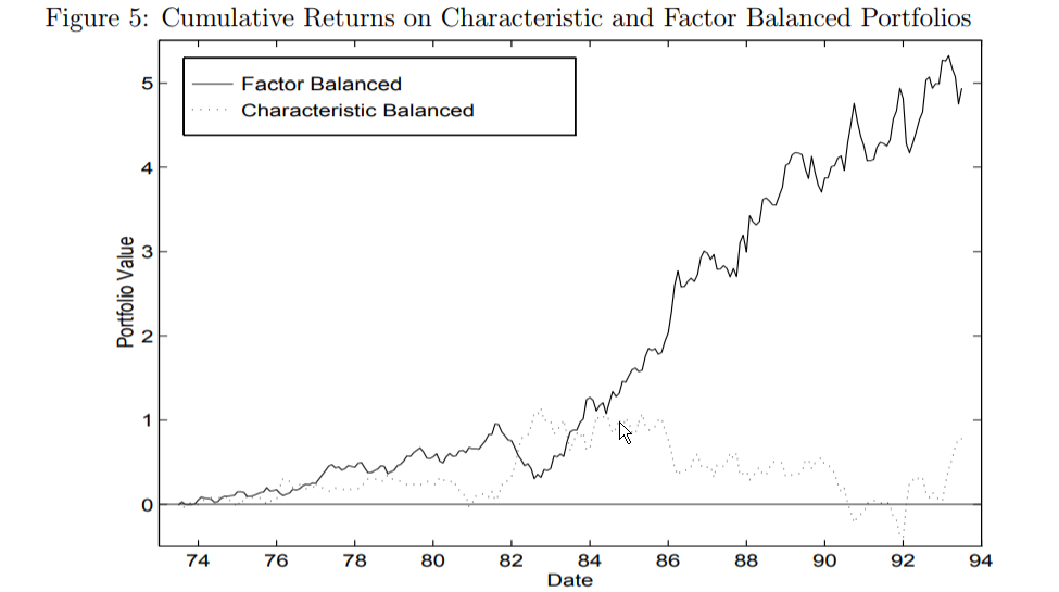
The evidence from the primary set of papers (here and here) strongly suggests that investors should focus on characteristics, not factors. The chart below summarizes the debate. The “factor balanced” portfolio is a long/short portfolio where both legs have similar factor loadings but the long leg has stronger characteristics than the short leg. The “characteristic balanced” portfolio is a portfolio where the long and short have different factor loadings but similar characteristics.
Summary: characteristics matter, whereas factor loadings do not.
The results are hypothetical results and are NOT an indicator of future results and do NOT represent returns that any investor actually attained. Indexes are unmanaged, do not reflect management or trading fees, and one cannot invest directly in an index. Additional information regarding the construction of these results is available upon request.
As we’ll show, the debate is arguably not as clear as the chart above suggests, and academics have argued over the interpretation of the value premium for almost 25 years. Why? The argument driving the value premium underlies core arguments related to how markets work — a fundamental question we still don’t completely understand.
A summary of each argument is described below:(1)
- The risk theory says value stocks are inherently riskier due to loading on an unknown distress factor. Since they are riskier, investors should demand a higher rate of return for taking on additional risk. Under this model, the value premium will continue to exist as long as investor risk preferences stay the same; however, if investor risk preferences change and they are willing to take on additional risk for a lower rate of return (unlikely!), the value premium will go away.(2).
- The LSV behavioral theory is a mispricing theory that claims that investors incorrectly extrapolate past growth rates (behavioral error) and cause value stocks to be under-priced and growth stocks to be over-priced–this causes the future higher (lower) returns to value (growth) stocks.
Under this model, the value premium will continue to exist as long as investors continue to make behavioral errors and the limits to arbitrage exist–we give a deep explanation of this model here. However, the value premium may disappear if investors stop making behavioral errors and the limits to arbitrage disappear.(3)
The characteristic theory claims that characteristics explain the cross-section of stock returns and that value firms had higher returns due to having a certain characteristic, such as a high B/M ratio. What are the implications of this model? Directly from the last paragraph of the 1997 Daniel and Titman paper:(4)
Another possibility is that investors consistently held priors that size and book-to-market ratios were proxies for systematic risk and, as a result, attached higher discount rates to stocks with these characteristics. … If this is the case, then the patterns we have observed in the data should not be repeated in the future.
So what’s the answer? A new paper entitled, “Interpreting Factor Models,” says it best:
We argue that tests of reduced-form factor models and horse races between “characteristics” and “covariances'” cannot discriminate between alternative models of investor beliefs.
In short, nobody knows.
We would argue that there is a mix of all three ideas simultaneously. As more investors learn about an investment approach that previously had higher returns (value investing), the expected returns to that approach may diminish in the future (implication of the characteristic theory), if arbitrage constraints are minimal.(5)
The rest of the article is broken into three sections:
- A dive into the characteristic versus risk debate.
- An examination of what this means for a long-only value investor
- A review of live portfolios with a breakdown of factors and characteristics
Let’s dig into the debate on factors vs characteristics.
A PDF version of this is available here.
Do Portfolio Factors or Characteristics Drive Expected Returns?
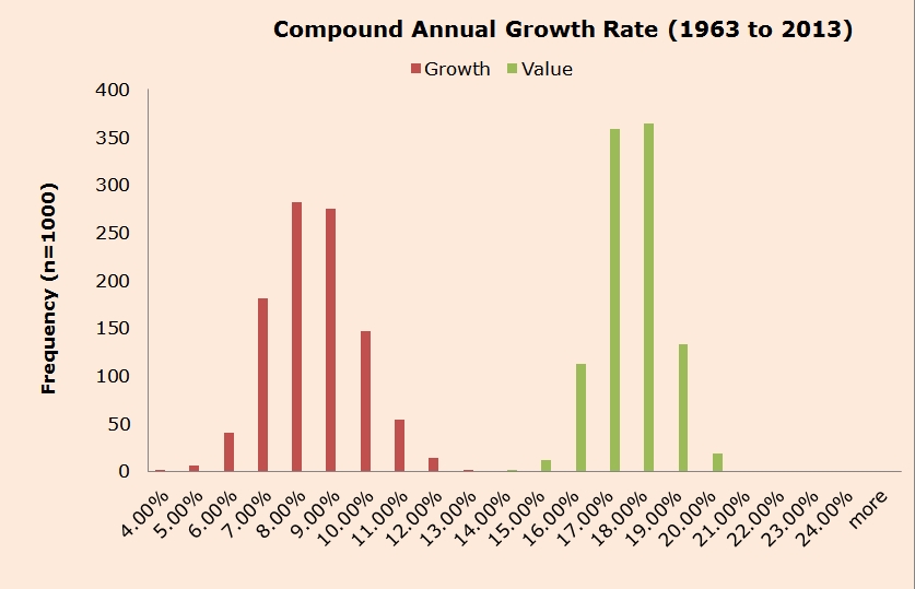
Most in finance are aware of the value premium: Historically, cheap stocks have outperformed expensive stocks (based on some price to fundamental). Below is a chart from a simulation exercise that highlights the performance of cheap vs. expensive portfolio simulations from 1963 to 2013.
The results are hypothetical results and are NOT an indicator of future results and do NOT represent returns that any investor actually attained. Indexes are unmanaged, do not reflect management or trading fees, and one cannot invest directly in an index. Additional information regarding the construction of these results is available upon request.
This concept is central to the debate about factors vs. characteristics.
One of the original papers on the value premium topic was Fama and French in 1993. Their paper finds that three factors (the market, size, and value proxied by Mkt_rf, SMB, and HML) explain the cross-section of stock returns. More important to this discussion, they suggest that value is a risk factor, as value firms covary with one another. In their story, the covariance matters, which is why the loading on HML is important.(6)
But what are some implications of this theory? Directly from FF 1993:
The regression slopes and the historical average premiums for the factors can then be used to estimate the (unconditional) expected return for the portfolio.
In other words, the HML loading can estimate future expected returns. A higher loading implies a higher risk, which implies a higher expected return rate. This is exactly the interpretation we often hear from DFA advisors, many of whom have been taught by Fama and French.
But the factor approach (and the reliance on regression slopes to make decisions) is not a panacea and has plenty of holes like any other approach.
We have discussed in detail, an alternative explanation to risk being the driver of the value premium is the LSV behavioral theory. The LSV theory suggests that investors over-extrapolate data, causing prices to sometimes deviate from fundamentals, and limits to arbitrage prevent these mispricings from being “arbitraged” away.
It is important, for this discussion, to note that the argument between the risk and LSV behavior camps does not focus on whether or not a factor model can explain the return premia of value and small firms–they agree it can. However, they argue whether the factors represent an economically relevant risk or mispricing that is costly to exploit.
However, there is a 3rd explanation for the value premium, which is also a “mispricing” based argument–the premium is simply driven by characteristics (not covariances, or factors). In other words, your HML loading does NOT matter, but your portfolio book-to-market ratio does matter.
Why Characteristics Matter: The Theory
This theory was proposed by Kent Daniel and Sheridan Titman in 1997, in their paper titled “Evidence on the Characteristics of Cross Sectional Variation in Stock Returns.”(7)(8)
This is a well-written paper. The introduction very clearly states what the paper will test, and what they find:
In contrast, this article addresses the more fundamental question of whether the return patterns of characteristic-sorted portfolios are really consistent with a factor model at all. Specifically, we ask (1) whether there really are pervasive factors that are directly associated with size and book-to-market; and (2) whether there are risk premia associated with these factors. In other words, we directly test whether the high returns of high book-to-market and small size stocks can be attributed to their factor loadings.Our results indicate that (1) there is no discernible separate risk factor associated with high or low book-to-market (characteristic) firms, and (2) there is no return premium associated with any of the three factors identified by Fama and French (1993), suggesting that the high returns related to these portfolios cannot be viewed as compensation for factor risk…Once we control for firm characteristics, expected returns do not appear to be positively related to the loadings on the market, HML, or SMB factors.
So what this paper is trying to argue is that after controlling for characteristics, factor exposures (i.e., factor “loadings”) don’t tell us much about expected returns. In other words, if an investor is calculating “HML loadings” to tell them something about future returns, they should stop this practice. Instead, investors should identify the book-to-market ratio of their portfolio, which will be much more predictive of expected returns.
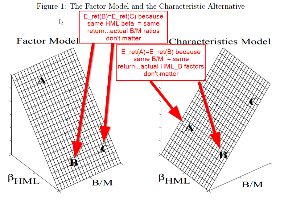
Before digging into Daniel and Titman’s 1997 Journal of Finance paper, I will quote and use a few images from their 1998 Journal of Portfolio Management paper, which nicely explains their argument. This paper can be found here and a working paper (used below) can be found here. Consider that we have three stocks: A, B, and C. Here are the assumed facts about these securities:
- Stock A and stock B have the same B/M ratio
- Stock A has a higher HML loading (
) than stock B.
- Stock C has a higher B/M ratio than stock B.
- Stock B and stock C have the same HML loading (
).
Figure 1 highlights the facts, and the arguments for the factor model versus the characteristic model. The y-axis in this image is expected returns. As can be seen in the left image, if the factor model is correct, then firms with the same , such as firms B and C, should have the same expected return. On the other hand, A has a higher
than B or C, which implies that A should have a higher expected return, according to the factor model. Now the right image documents the characteristic model. Here, stocks A and B have the same B/M ratio, so they should have the same expected return. Since C has a higher B/M ratio than A and B, it should have a higher expected return. according to the characteristic model.
Why Characteristics Matter: The Evidence
In the 1997 paper, the authors form 45 portfolios to test their idea that characteristics are better than factors (covariances). The form portfolios employ a 3-way split. They first split firms into three groups of size and B/M, yielding nine portfolios. Within each of the nine portfolios, they split firms into five groups based on their HML loading, yielding 45 portfolios. Table IV of the 1997 paper highlights shows the 45 portfolios, first split on size and B/M, then on HML.(9)
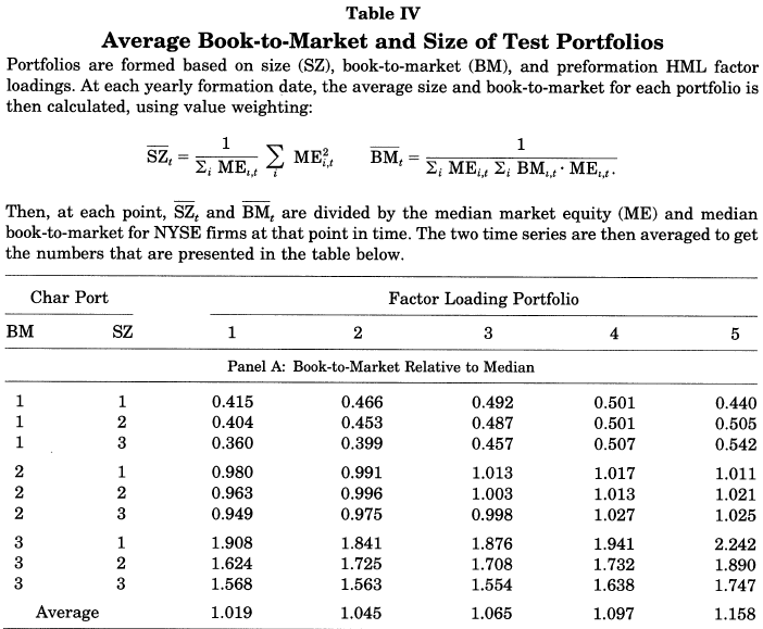
The results are hypothetical results and are NOT an indicator of future results and do NOT represent returns that any investor actually attained. Indexes are unmanaged, do not reflect management or trading fees, and one cannot invest directly in an index. Additional information regarding the construction of these results is available upon request. From “Evidence on the Characteristics of Cross Sectional Variation in Stock Returns” by Kent Daniel and Sheridan Titman (1993). http://www.kentdaniel.net/papers/published/jf97.pdf
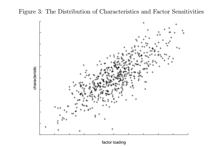
How does one test the characteristic model against the factor model when characteristics and factors are so correlated?(10)
The authors build what they call characteristic balanced portfolios based on HML loadings.(11)
For each of the nine portfolios split on size and B/M, the authors go long the top two portfolios on the HML loadings and short the bottom two portfolios on the HML loadings. In the end, each portfolio has similar characteristics, such as size and B/M ratios, but the HML dimension can vary.(12)
What would the factor model predict versus the characteristics model for these portfolios?
The factor model would suggest the following:
- The L/S portfolio should have positive expected returns because the portfolios are long the high HML firms and short the low HML firms.
- Alpha should be zero because the Fama and French 3-factor model will pick up the variation in returns via a higher HML loading.
The characteristic model predicts something different:
- The L/S should have flat expected returns because the portfolios are formed with similar characteristics (Size and B/M).
- Alpha could be positive because the 3-factor model may not fully pick up the variation in returns due to characteristics.
Table VI of the paper highlights the main takeaway. As shown below, the combined portfolio, which is long high HML firms and short low HML firms, while controlling for the characteristics, has a positive and significant 3-factor alpha. In addition, from the text of the paper, the mean return to this portfolio is -0.116% per month, and is not significantly different from zero (t-stat of -0.60).
The evidence supports the characteristics model’s predictions: Controlling for characteristics, factor loadings don’t matter.
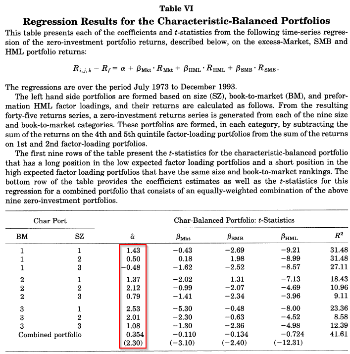
The results are hypothetical results and are NOT an indicator of future results and do NOT represent returns that any investor actually attained. Indexes are unmanaged, do not reflect management or trading fees, and one cannot invest directly in an index. Additional information regarding the construction of these results is available upon request. From “Evidence on the Characteristics of Cross Sectional Variation in Stock Returns” by Kent Daniel and Sheridan Titman (1993). Accessed from: http://www.kentdaniel.net/papers/published/jf97.pdf
The results additionally hold for the SMB and Mkt_RF loadings, which are once again consistent with the characteristic model. These results are shown in Tables VII and VIII of the 1997 paper. The above portfolios are characteristically balanced.
But what about factor balanced portfolios?
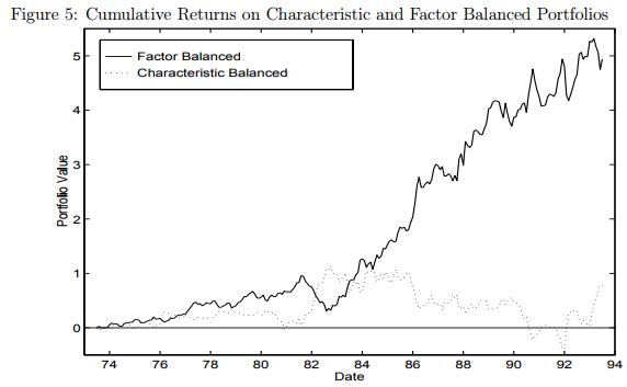
This analysis is done in the 1998 JPM paper. They compare the returns of the characteristic balanced portfolios against the factor balanced portfolios. Factor balanced portfolios are now balanced along the dimensions of factors. These portfolios load 0 on each of the three factors (market, size, and value), while they vary along the characteristic dimensions (size and B/M).
We have two portfolios to test in our analysis of factors vs. characteristics:
- Characteristic Balanced: Long high HML firms and short low HML firms, controlling for characteristics
- Factor Balanced: Long high B/M firms and short low B/M firms, controlling for factor loadings (market, size, and value).
The results are shown in Figure 5 of the 1998 paper, and are shown below:
The results are hypothetical results and are NOT an indicator of future results and do NOT represent returns that any investor actually attained. Indexes are unmanaged, do not reflect management or trading fees, and one cannot invest directly in an index. Additional information regarding the construction of these results is available upon request. From “Characteristics or Covariances?” by Daniel and Titman. Accessed 10/23/17 from: http://www.kentdaniel.net/papers/published/jpm_98.pdf
This image of the cumulative returns highlights two things:
- Controlling for characteristics, factor loadings do not matter.
- Controlling for loadings, characteristics do matter.
Bottom line on factors vs characteristics: Focus on your portfolio characteristics, not your portfolio factor loadings!
Fama and French Fight Back
Why is everyone still using factor models in 2017? Well, the debate didn’t end with Daniel and Titman 1997. In 2000, James Davis, Eugene Fama, and Ken French (DFF) came to defend factor models. Their paper is titled, “Characteristics, Covariances, and Average Returns: 1929-1997.”(13) DFF run similar tests as the DT paper, but over a longer time cycle. A minor portfolio construction change is made by creating 27 portfolios instead of 45. Like DT, DFF first split the universe into nine portfolios based on size and B/M ratios. Next, for each of the nine portfolios split on size and B/M, the authors split the firms into three groups along the HML loadings, leading to 27 portfolios. Within each of the nine portfolios sorted on size and B/M, DFF go long the high HML firms and short the low HML firms.
As a reminder, here is what the two models would predict (from above):
The factor model would say the following:
- The mean monthly return should be positive, as the portfolios are long the high HML firms and short the low HML firms.
- The mean alpha should be zero, as the 3-factor model should pick up the variation in returns via a higher HML loading.
The characteristic model would say the following:
- The mean monthly return should be zero, as the portfolios are formed by controlling for the characteristics (Size and B/M).
- The mean alpha should be positive, as the 3-factor model may not fully pick up the variation in returns due to characteristics.
The results are shown in Table IV of the DFF paper and below:
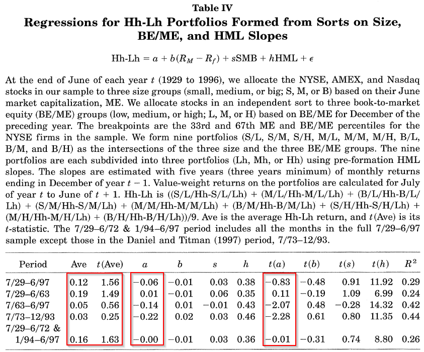
The results are hypothetical results and are NOT an indicator of future results and do NOT represent returns that any investor actually attained. Indexes are unmanaged, do not reflect management or trading fees, and one cannot invest directly in an index. Additional information regarding the construction of these results is available upon request. From “Characteristics or Covariances: Evidence from 1927-1997: by Davis, Fama, and French. Accessed on 10/23/17 from: https://www8.gsb.columbia.edu/sites/valueinvesting/files/files/06davis_fama_french_2000_29-97.pdf
Examining the first (full-time period) and last row (full-time period excluding the DT time period), we find that the results are consistent with the factor model. The average return is positive and significant, while the alpha is insignificantly different than zero. This is different than the time period studied in the JT paper, which was July of 1973-December 1993. During that time period, DFF find the results consistent with the characteristic model–the average return is insignificantly different than zero and there is a significant alpha not picked up by the 3-factor model.
So, in conclusion, DFF finds that over the entire sample, the results are more consistent with the factor model, whereas the results from the DT paper may be specific to a certain time period. Thus, factor models are saved!
So is that the end of the story? Not exactly.
Out-of-Sample Studies to Settle the Factors vs Characteristics Debate
Two additional studies conduct the same tests, out of sample, by using returns from Japan and the U.K.
The abstract from a 2001 paper titled, “Explaining the Cross-Section of Stock Returns in Japan: Factors or Characteristics” by Kent Daniel, Sheridan Titman, and K. C. John Wei.
Japanese stock returns are even more closely related to their book-to-market ratios than are their U.S. counterparts, and thus provide a good setting for testing whether the return premia associated with these characteristics arise because the characteristics are proxies for covariance with priced factors. Our tests, which replicate the Daniel and Titman [1997] tests on a Japanese sample, reject the Fama and French [1993] three-factor model, but fail to reject the characteristic model.
The abstract from a 2007 paper titled, “UK Evidence on the Characteristics versus Covariance Debate” by Edward Lee, Weimin Liu, and Norman Strong.
We evaluate the Fama–French three-factor model in the UK using the approach of Daniel and Titman (1997) to determine whether characteristics or covariance risk better explains the size and value premiums. Across all three factors, we find that return premiums bear little relationship to the corresponding loadings. We show that small and value stocks earn higher returns irrespective of their return covariance. Our study contributes to the existing literature by reporting original findings on the Fama–French three-factor model in the UK and by reporting results that complement existing evidence from similar studies in the USA and Japan.
So in two out-of-sample datasets, the evidence favors the characteristic model.(14)
What do we make of all this, and what does it mean for our discussion of factors vs characteristics?
First off, factor models are just that– a model. It should be pointed out that many still examine and give weight to the beta of a portfolio, which is built upon the portfolio’s covariance relative to the market’s variance. A higher beta should imply higher returns–we know that is not necessarily the case. Additionally, saying that the HML loading of a portfolio is unrelated to the B/M of the portfolio is untrue as well–the HML factor creates a long/short portfolio return by sorting stocks on B/M!
So, in the end, it is hard to ascertain which is 100% correct. In the end, both characteristics and loadings probably matter when explaining the cross-section of stock returns.
But how does this affect a long-only value investor? Below I examine this question directly.
I’m Not From the Ivory Tower: How Does This Affect My Clients and Me?
While the analysis above is an academic debate within long/short portfolios, what are the implications for a long-only investor interested in a particular investment approach, such as Value and Momentum investing? Below I examine this in the context of a Value investor by allowing portfolios to be split into Value-Growth Deciles by two methods:
- The previous HML loading.
- The B/M ratio.
The HML loading for each stock is the Beta on the HML factor from Ken French’s website from a regression on the 4-factor model over the past 36 months.(15) Stocks without 36 months of past returns are eliminated from the sample. Similarly, stocks without B/M ratios are also eliminated from the sample. Last, I exclude firms below the 40th percentile of NYSE market capitalization, to eliminate small and micro-cap stocks from the sample, and focus mainly on mid/large-cap firms. Portfolios are formed annually on 6/30 each year, and the returns are examined from 7/1 of year t to 6/30 of year t+1. Compound Annual Growth Rates (CAGRs) are measured from 7/1/1973 – 12/31/2016 and are shown below, gross of any fees or transaction costs.(16) For reference, over this time period, the VW and EW Universe returned 10.80% and 13.18%, respectively, while the SP500 and Sp500 EW returned 10.69% and 13.66% respectively, gross of any fees or transaction costs.(17)
VW Returns: 7/1/1973 – 12/31/2016
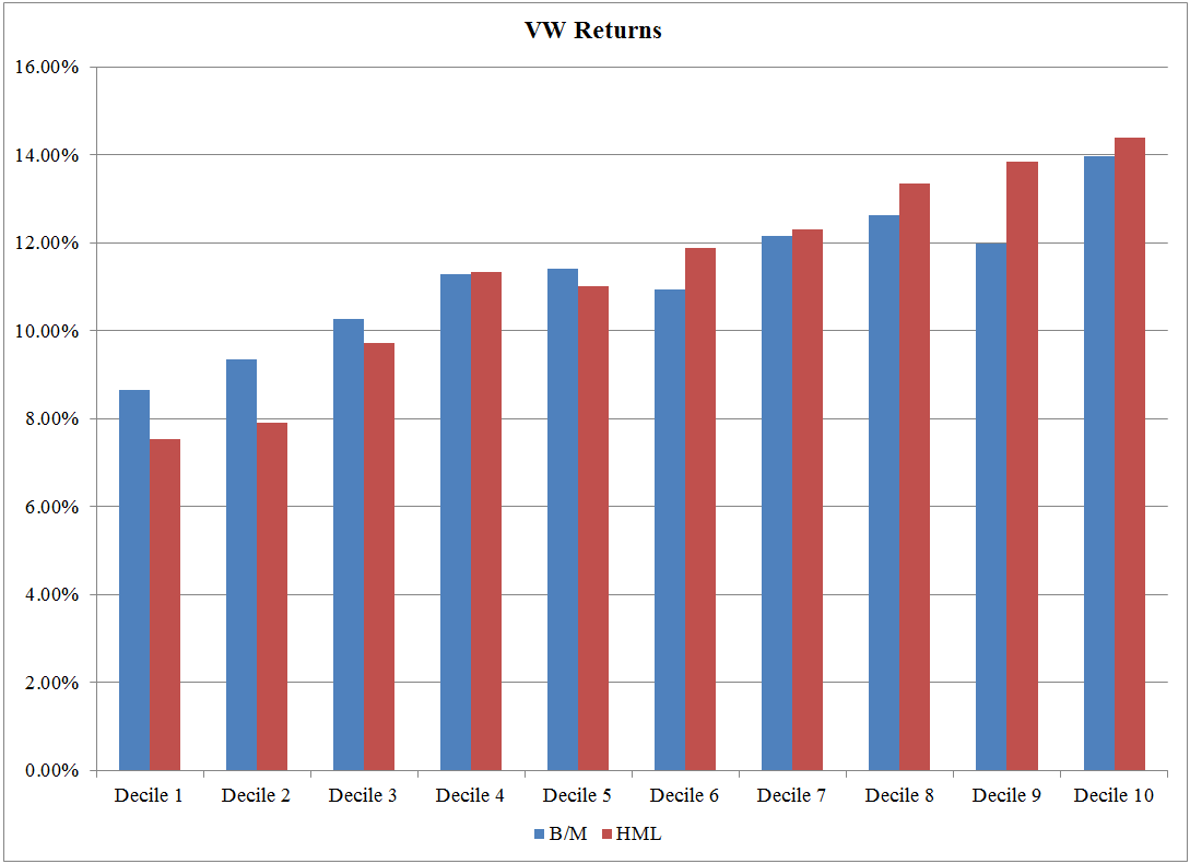
The results are hypothetical results and are NOT an indicator of future results and do NOT represent returns that any investor actually attained. Indexes are unmanaged, do not reflect management or trading fees, and one cannot invest directly in an index.
As seen in the image above, the CAGRs for the portfolios increase for both the HML deciles and the B/M deciles as one moves from Growth to Value firms (left to right). This highlights that using characteristics (B/M) and factors (HML loadings) to create Value portfolios worked in the past, as the Value decile outperformed the Growth decile. Given the evidence in our charts and the papers above, most long-only investors find it hard to argue that sorting a portfolio on characteristics is a bad way to form value portfolios. Across each decile, the correlation between the portfolios formed on B/M and HML loadings is high and range between 0.86 and 0.925. It should be noted that the high B/M and HML decile portfolios (both VW and EW) have a tracking error relative to the SP500 of at least 10%, so these are portfolios that many professional money managers would not use (too much career risk!).
Sub-period analysis is done and shown in the below reference–it is generally found that characteristics performed better in the original DT sample period (7/1/1973-12/31/2016), whereas forming portfolios on HML performed better (especially for the VW portfolios) in the period after that (1/1/1994-12/31/2016).(18)
But given that we have the data, what are the loadings of the Value portfolios formed either by sorting on
B/M ratios or by HML loadings?
Below we show the 4-factor loadings over the entire time period tested above (7/1/1973-12/31/12016):
| 4-Factor Regression | ||||||
| Alpha (Annual) | MKT_RF | SMB | HML | MOM | ||
| High HML VW | 4-Factor | 0.00 | 1.17 | 0.10 | 0.60 | 0.00 |
| p-value | 0.8907 | 0.0000 | 0.0574 | 0.0000 | 0.9542 | |
| High B/M VW | 4-Factor | 0.00 | 1.05 | 0.04 | 0.78 | -0.15 |
| p-value | 0.7484 | 0.0000 | 0.2746 | 0.0000 | 0.0000 | |
| High HML EW | 4-Factor | 0.00 | 1.12 | 0.36 | 0.58 | 0.00 |
| p-value | 0.9423 | 0.0000 | 0.0000 | 0.0000 | 0.9055 | |
| High B/M EW | 4-Factor | 0.02 | 1.01 | 0.25 | 0.71 | -0.15 |
| p-value | 0.7484 | 0.0000 | 0.0000 | 0.0000 | 0.0000 |
The results are hypothetical results and are NOT an indicator of future results and do NOT represent returns that any investor actually attained. Indexes are unmanaged, do not reflect management or trading fees, and one cannot invest directly in an index.
This can be important for the analysis by advisors on certain funds. Let’s say, as an advisor, you want to assess a fund that claims to sort firms on P/E ratios.(19)
Well, almost by construction, sorting firms on P/E will most likely (but not always) lead to a lower HML, or “value” loading, than another fund that sorts on B/M.(20) So does this mean that the P/E fund is not a value fund as it doesn’t have a high HML loading? Not necessarily; one way to ascertain what the P/E fund is doing is to examine the portfolio’s characteristics. Similarly, how can one assess a multi-factor fund? Without tools to assess the portfolio, it can be tough to decide.
Let’s examine a live portfolio and highlight the factor loadings and the overlap to the academic value portfolio formed on characteristics. We will then discuss a new tool we plan to launch soon, which will help advisors assess the characteristics of an ETF or even a portfolio of ETFs.
Examination of a live portfolio
To examine both the factor loadings, as well as the portfolio characteristics, I chose Vanguard’s VTV ETF. A huge “value” ETF known to most professional investors.
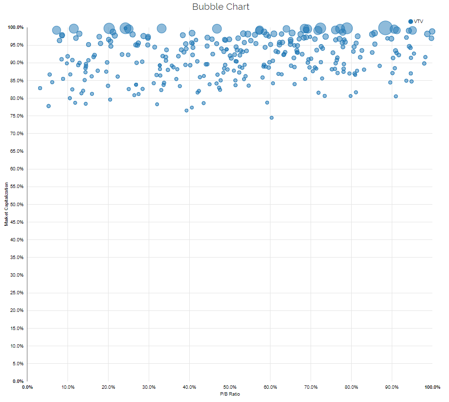
To examine the factor loadings, I use the online tool, PortfolioVisualizer. A link can be found here and an image of the factor loadings to VTV is shown below:
As seen above, the fund’s loadings are 0.97 on the market, a negative 0.19 loading on SMB, and a positive 0.27 loading on HML–all are significant. Since this is a value fund, where the positions are mainly value-weighted (market-cap weighted), these loadings make sense–market beta ~ 1 as it market-cap weights large stock positions, a negative size loading as it invests in large stocks, and a positive HML loading as it is a Value fund. So nothing surprising here.
Next, we examine this same ETF using our Visual Active Share tool–an explanation of this tool can be found here. Our tool allows an investor to analyze a fund from a characteristics-based framework instead of a regression/factor-based framework.
On the image above, each circle represents an underlying stock, with the size of the circle representing the weight of the stock within the ETF. The x-axis ranks all non-micro-cap stocks on P/B (inverse of B/M), while the y-axis ranks all stocks on size. As shown above, VTV is a larger cap fund, as the holdings are ~ 75th percentile and higher, emphasizing the largest stocks in the universe. The Fund seems to have little relationship with P/B, as the dots are spread across the spectrum of cheap/expensive.
Let’s dig further.
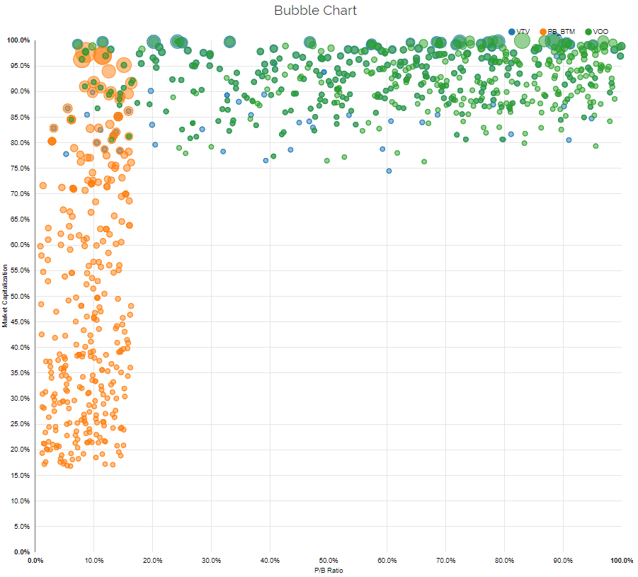
How does VTV compare to “academic” value portfolios, formed on characteristics? Within the visual active share tool, we have the academic characteristic portfolios pre-built (start typing “academic” and they’ll show up). Below we add the academic bottom decile on P/B (inverse of B/M), where a lower P/B indicates a firm is cheaper. We also add Vanguard’s SP500 ETF, VOO to view the index holdings.
As seen above, the VTV and VOO ETFs (Value and SP500) hold very similar positions. The fee difference is 0.02%, so one can’t complain about the funds being too similar (you aren’t paying for any differentiation). Also, one notices that these funds differ from the academic characteristic-based P/B portfolio. This makes sense–Vanguard gives investors access to the market-cap portfolio, for a very cheap price. They are not trying to be that different than the market, and by doing so, have helped many investors. But clearly, this fund is not the same as the characteristic-based academic portfolio. Our Visual Active Share tool can be helpful to visually view the differences between live funds and the characteristic-based academic portfolio.
(21)Bottom line: We’re building out a capability for investors to assess portfolios based on characteristics instead of factors.
Concluding thoughts on factors vs characteristics
We started this discussion about factors vs characteristics by highlighting the perpetual debate regarding the value premium–risk or mispricing? We introduced an alternative way of viewing the world via characteristics-based asset pricing.
The main takeaways are the following:
- There is a clear academic debate about whether factors or characteristics drive higher returns to value and small firms. There is decent evidence to suggest that both models have legs to stand on, which implies the future expected return to the value premium. However, it should be noted that the two are clearly related–the HML is formed by sorting firms on size and B/M, so an HML loading has some relation to the B/M characteristic. We don’t necessarily take a side here, but rather highlight that one can examine both loadings and characteristics to assess a fund.
- When assessing the returns to value paper portfolios, sorting on either factors or characteristics yielded a similar result from a CAGR and ex-post factor loading perspective. Thus, examining the current characteristics of portfolios is not a bad idea.
- We walked through an example of a value fund and highlighted our Visual Active Share tool, which allows investors to view underlying stocks along different characteristics.
Overall, factor investing comes in many shades. While factor loadings can be important, examining characteristics is arguably just as effective (and probably more intuitive!).
In the end, factor investing is more art and less science.
References[+]
| ↑1 | Note — a 4th explanation of the value premium is that it was a chance result, and is unlikely to be found out of sample. However, the out-of-sample data contradicts this idea. Value and Momentum have been found to work (almost) everywhere. |
|---|---|
| ↑2 | Note that if investors decide to purchase value stocks, regardless of risk, this could diminish the premium |
| ↑3 | We believe the largest cost of arbitrage is tracking error risk, which is further explained in this paper on “Interpreting Factor Models.“ |
| ↑4 | This can be viewed as mispricing theory, or maybe not. |
| ↑5 | ”Fact, Fiction, and Value-investing” also outlines the argument that there probably isn’t a catch-all explanation for factor premiums. |
| ↑6 | As a reminder, a stock’s market Beta is a measure of the firm’s covariance with the market, divided by the variance of the market. |
| ↑7 | I highly recommend everyone read the entire paper. |
| ↑8 | A great replication and explanation of this paper, as well as the source code, was done by Alex Chinco and can be found here. |
| ↑9 | A pretty version of this analysis is here. |
| ↑10 | (see table below from 1998 paper). This is a critical part of the factor vs. characteristics debate.
 https://alphaarchitect.com/wp-content/uploads/2017/11/2017-10-31-08_02_44-D__kent_proj_jpm_jpm6.DVI_-200x139.png 200w, https://alphaarchitect.com/wp-content/uploads/2017/11/2017-10-31-08_02_44-D__kent_proj_jpm_jpm6.DVI_-400x277.png 400w, https://alphaarchitect.com/wp-content/uploads/2017/11/2017-10-31-08_02_44-D__kent_proj_jpm_jpm6.DVI_-600x416.png 600w, https://alphaarchitect.com/wp-content/uploads/2017/11/2017-10-31-08_02_44-D__kent_proj_jpm_jpm6.DVI_-800x555.png 800w, https://alphaarchitect.com/wp-content/uploads/2017/11/2017-10-31-08_02_44-D__kent_proj_jpm_jpm6.DVI_.png 844w" sizes="(max-width: 844px) 100vw, 844px" /> https://alphaarchitect.com/wp-content/uploads/2017/11/2017-10-31-08_02_44-D__kent_proj_jpm_jpm6.DVI_-200x139.png 200w, https://alphaarchitect.com/wp-content/uploads/2017/11/2017-10-31-08_02_44-D__kent_proj_jpm_jpm6.DVI_-400x277.png 400w, https://alphaarchitect.com/wp-content/uploads/2017/11/2017-10-31-08_02_44-D__kent_proj_jpm_jpm6.DVI_-600x416.png 600w, https://alphaarchitect.com/wp-content/uploads/2017/11/2017-10-31-08_02_44-D__kent_proj_jpm_jpm6.DVI_-800x555.png 800w, https://alphaarchitect.com/wp-content/uploads/2017/11/2017-10-31-08_02_44-D__kent_proj_jpm_jpm6.DVI_.png 844w" sizes="(max-width: 844px) 100vw, 844px" /> |
| ↑11 | This term is used in the 1998 JPM paper, but is instructive so I use it here. |
| ↑12 | Again, this portfolio sort is possible because there are groups of cheap small-cap value stocks with high HML betas, and there are groups of cheap small-cap value stocks with low HML betas. |
| ↑13 | Note the dates are included in the title of the paper–a big chunk of the paper is devoted to highlighting that the Daniel and Titman results are very specific to the time period tested in the DT paper — 1973-1993. |
| ↑14 | Here is a paper that examines mutual fund portfolios using characteristic-based benchmarks–this is one way to assess mutual funds and ETFs. |
| ↑15 | Regression of excess stock returns against the market-risk free, SMB, HML, and MOM factors. |
| ↑16 | Manager Fees and transaction costs would lower the returns to each of the decile portfolios |
| ↑17 |
EW Returns: 7/1/1973 – 12/31/2016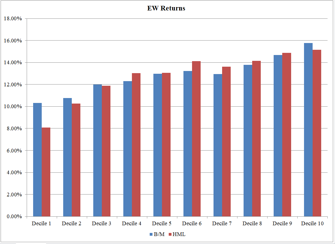 https://alphaarchitect.com/wp-content/uploads/2017/08/factors-or-characteristics.7-200x145.png 200w, https://alphaarchitect.com/wp-content/uploads/2017/08/factors-or-characteristics.7-400x291.png 400w, https://alphaarchitect.com/wp-content/uploads/2017/08/factors-or-characteristics.7-600x436.png 600w, https://alphaarchitect.com/wp-content/uploads/2017/08/factors-or-characteristics.7-800x582.png 800w, https://alphaarchitect.com/wp-content/uploads/2017/08/factors-or-characteristics.7.png 1092w" sizes="(max-width: 1092px) 100vw, 1092px" /> https://alphaarchitect.com/wp-content/uploads/2017/08/factors-or-characteristics.7-200x145.png 200w, https://alphaarchitect.com/wp-content/uploads/2017/08/factors-or-characteristics.7-400x291.png 400w, https://alphaarchitect.com/wp-content/uploads/2017/08/factors-or-characteristics.7-600x436.png 600w, https://alphaarchitect.com/wp-content/uploads/2017/08/factors-or-characteristics.7-800x582.png 800w, https://alphaarchitect.com/wp-content/uploads/2017/08/factors-or-characteristics.7.png 1092w" sizes="(max-width: 1092px) 100vw, 1092px" />The results are hypothetical results and are NOT an indicator of future results and do NOT represent returns that any investor actually attained. Indexes are unmanaged, do not reflect management or trading fees, and one cannot invest directly in an index. |
| ↑18 |
VW Returns: 7/1/1973 – 12/31/1993 https://alphaarchitect.com/wp-content/uploads/2017/08/factors-or-characteristics.8-1-200x146.png 200w, https://alphaarchitect.com/wp-content/uploads/2017/08/factors-or-characteristics.8-1-400x291.png 400w, https://alphaarchitect.com/wp-content/uploads/2017/08/factors-or-characteristics.8-1-600x437.png 600w, https://alphaarchitect.com/wp-content/uploads/2017/08/factors-or-characteristics.8-1-800x582.png 800w, https://alphaarchitect.com/wp-content/uploads/2017/08/factors-or-characteristics.8-1.png 1087w" sizes="(max-width: 1087px) 100vw, 1087px" /> https://alphaarchitect.com/wp-content/uploads/2017/08/factors-or-characteristics.8-1-200x146.png 200w, https://alphaarchitect.com/wp-content/uploads/2017/08/factors-or-characteristics.8-1-400x291.png 400w, https://alphaarchitect.com/wp-content/uploads/2017/08/factors-or-characteristics.8-1-600x437.png 600w, https://alphaarchitect.com/wp-content/uploads/2017/08/factors-or-characteristics.8-1-800x582.png 800w, https://alphaarchitect.com/wp-content/uploads/2017/08/factors-or-characteristics.8-1.png 1087w" sizes="(max-width: 1087px) 100vw, 1087px" />The results are hypothetical results and are NOT an indicator of future results and do NOT represent returns that any investor actually attained. Indexes are unmanaged, do not reflect management or trading fees, and one cannot invest directly in an index. EW Returns: 7/1/1973 – 12/31/1993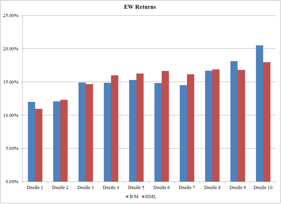 https://alphaarchitect.com/wp-content/uploads/2017/08/factors-or-characteristics.9-200x145.png 200w, https://alphaarchitect.com/wp-content/uploads/2017/08/factors-or-characteristics.9-400x291.png 400w, https://alphaarchitect.com/wp-content/uploads/2017/08/factors-or-characteristics.9-600x436.png 600w, https://alphaarchitect.com/wp-content/uploads/2017/08/factors-or-characteristics.9-800x582.png 800w, https://alphaarchitect.com/wp-content/uploads/2017/08/factors-or-characteristics.9.png 1088w" sizes="(max-width: 1088px) 100vw, 1088px" /> https://alphaarchitect.com/wp-content/uploads/2017/08/factors-or-characteristics.9-200x145.png 200w, https://alphaarchitect.com/wp-content/uploads/2017/08/factors-or-characteristics.9-400x291.png 400w, https://alphaarchitect.com/wp-content/uploads/2017/08/factors-or-characteristics.9-600x436.png 600w, https://alphaarchitect.com/wp-content/uploads/2017/08/factors-or-characteristics.9-800x582.png 800w, https://alphaarchitect.com/wp-content/uploads/2017/08/factors-or-characteristics.9.png 1088w" sizes="(max-width: 1088px) 100vw, 1088px" />The results are hypothetical results and are NOT an indicator of future results and do NOT represent returns that any investor actually attained. Indexes are unmanaged, do not reflect management or trading fees, and one cannot invest directly in an index. VW Returns: 1/1/1994- 12/31/2016 https://alphaarchitect.com/wp-content/uploads/2017/08/factors-or-characteristics.10-200x145.png 200w, https://alphaarchitect.com/wp-content/uploads/2017/08/factors-or-characteristics.10-400x290.png 400w, https://alphaarchitect.com/wp-content/uploads/2017/08/factors-or-characteristics.10-600x435.png 600w, https://alphaarchitect.com/wp-content/uploads/2017/08/factors-or-characteristics.10-800x580.png 800w, https://alphaarchitect.com/wp-content/uploads/2017/08/factors-or-characteristics.10.png 1089w" sizes="(max-width: 1089px) 100vw, 1089px" /> https://alphaarchitect.com/wp-content/uploads/2017/08/factors-or-characteristics.10-200x145.png 200w, https://alphaarchitect.com/wp-content/uploads/2017/08/factors-or-characteristics.10-400x290.png 400w, https://alphaarchitect.com/wp-content/uploads/2017/08/factors-or-characteristics.10-600x435.png 600w, https://alphaarchitect.com/wp-content/uploads/2017/08/factors-or-characteristics.10-800x580.png 800w, https://alphaarchitect.com/wp-content/uploads/2017/08/factors-or-characteristics.10.png 1089w" sizes="(max-width: 1089px) 100vw, 1089px" />The results are hypothetical results and are NOT an indicator of future results and do NOT represent returns that any investor actually attained. Indexes are unmanaged, do not reflect management or trading fees, and one cannot invest directly in an index. EW Returns: 1/1/1994- 12/31/2016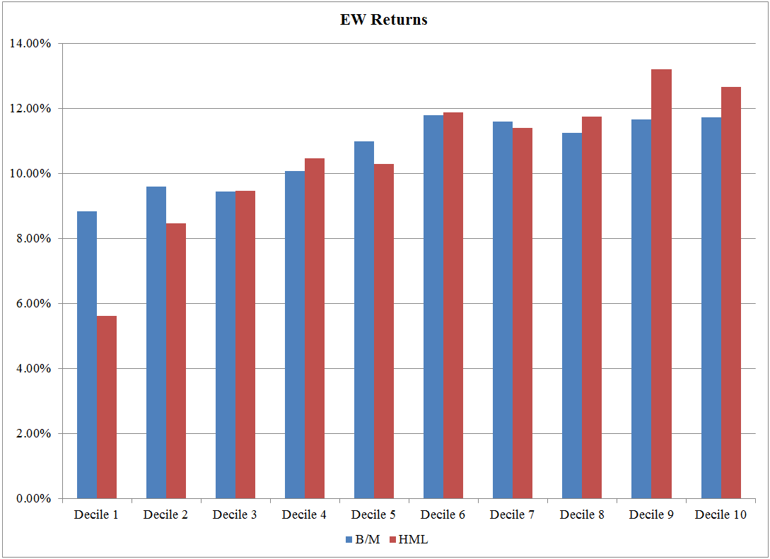 https://alphaarchitect.com/wp-content/uploads/2017/08/factors-or-characteristics.11-200x145.png 200w, https://alphaarchitect.com/wp-content/uploads/2017/08/factors-or-characteristics.11-400x291.png 400w, https://alphaarchitect.com/wp-content/uploads/2017/08/factors-or-characteristics.11-600x436.png 600w, https://alphaarchitect.com/wp-content/uploads/2017/08/factors-or-characteristics.11-800x581.png 800w, https://alphaarchitect.com/wp-content/uploads/2017/08/factors-or-characteristics.11.png 1089w" sizes="(max-width: 1089px) 100vw, 1089px" /> https://alphaarchitect.com/wp-content/uploads/2017/08/factors-or-characteristics.11-200x145.png 200w, https://alphaarchitect.com/wp-content/uploads/2017/08/factors-or-characteristics.11-400x291.png 400w, https://alphaarchitect.com/wp-content/uploads/2017/08/factors-or-characteristics.11-600x436.png 600w, https://alphaarchitect.com/wp-content/uploads/2017/08/factors-or-characteristics.11-800x581.png 800w, https://alphaarchitect.com/wp-content/uploads/2017/08/factors-or-characteristics.11.png 1089w" sizes="(max-width: 1089px) 100vw, 1089px" />The results are hypothetical results and are NOT an indicator of future results and do NOT represent returns that any investor actually attained. Indexes are unmanaged, do not reflect management or trading fees, and one cannot invest directly in an index. |
| ↑19 | Note we are big fans of Enterprise Multiples, as shown in our analysis here and here. |
| ↑20 | Assuming that P/E and B/M are not 100% correlated when sorting firms, this P/E fund will likely have a lower HML loading. |
| ↑21 | While this is a nice tool, we have had two common requests from those using the tool:
We are working on building these tools out now! The new tools will allow advisors to view the average characteristics of the ETFs–an example being the average Enterprise multiple being 10% for fund A and 6% for the Sp500. We will do this by calculating the value-weighted average for each characteristic. The second tool will allow advisors to build a portfolio of ETFs, and then view the overall overlap (relative to some index) as well as the average characteristics (P/E, Momentum, expense ratio, etc.) of the portfolio. So in total, we will have three tools that will allow advisors to better assess the characteristics of ETFs and portfolios of ETF. |
About the Author: Jack Vogel, PhD
—
Important Disclosures
For informational and educational purposes only and should not be construed as specific investment, accounting, legal, or tax advice. Certain information is deemed to be reliable, but its accuracy and completeness cannot be guaranteed. Third party information may become outdated or otherwise superseded without notice. Neither the Securities and Exchange Commission (SEC) nor any other federal or state agency has approved, determined the accuracy, or confirmed the adequacy of this article.
The views and opinions expressed herein are those of the author and do not necessarily reflect the views of Alpha Architect, its affiliates or its employees. Our full disclosures are available here. Definitions of common statistics used in our analysis are available here (towards the bottom).
Join thousands of other readers and subscribe to our blog.


