This blog talks about reinforcement learning for trading applications.
Once one of my pups found half a roast chicken in the corner of a parking lot and we had to visit that exact same corner every day for about fifty years because for dogs hope springs eternal when it comes to half a roast chicken – darth
Properly used, positive reinforcement is extremely powerful. – B. F. Skinner
Tic-Tac-Toe is a simple game. If both sides play perfectly, neither can win. But if one plays imperfectly, the other can exploit the flaws in the other’s strategy.
Does that sound a little like trading?
Reinforcement learning is a machine learning paradigm that can learn behavior to achieve maximum reward in complex dynamic environments, as simple as Tic-Tac-Toe, or as complex as Go, and options trading.
In this post, we will try to explain what reinforcement learning is, share code to apply it, and references to learn more about it.
- First, we’ll learn a simple algorithm to play Tic-Tac-Toe, then learn to trade a non-random price series.
- Finally, we’ll talk about how reinforcement learning can master complex financial concepts like option pricing and optimal diversification.
Let’s dive in!
A Tic-Tac-Toe example
What is reinforcement learning? Here’s a simple algorithm that will learn an exploitive Tic-Tac-Toe strategy, and adapt over time if its opponent learns:
- Make a big table of all possible Tic-Tac-Toe boards.
- Initialize the table to assign a value of 0 to each board, 1.0 where X has won, -1.0 where O has won.
- Play with your opponent. At each move, pick the best available move in your table, or if several are tied, pick one at random. Occasionally, make a move at random just to make sure you explore the whole state space, and to keep your opponent on their toes.
- After each game, back up through all the boards that were played.
Update the value table as follows:
- When X wins, update each board’s value part of the way to 1.
- When O wins, update part of the way to -1.
- When they tie, update part of the way to 0.
This is a profoundly dumb algorithm in the finest sense. It knows almost nothing about the dynamics of Tic-Tac-Toe, but it works. It can’t reason about the game. It needs a lot of training. It can’t generalize to boards it hasn’t seen.(1) It doesn’t learn a globally optimal strategy, it just tries to find whatever beats its opponent.
But over time, this algorithm learns, it exploits flaws in its opponent’s strategy, and if the opponent changes tactics, it adapts.
This is reinforcement learning.
More sophisticated reinforcement learning algorithms enable robots to walk on four or two legs, driverless cars to drive, computers to play Atari and poker and Go and StarCraft and DOTA and online soccer, in some cases better than humans.
Here is some sample Tic-Tac-Toe code. In this post, we’ll extend the Tic-Tac-Toe example to deep reinforcement learning, and build a reinforcement learning trading robot.
Key concepts
But first, let’s dig a little deeper into how reinforcement learning in general works, its components, and variations.
Figure 1. Markov Decision Process (MDP)
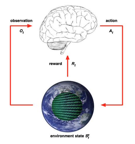
This figure and a few more below are from the lectures of David Silver, a leading reinforcement learning researcher known for the AlphaGo project, among others.
- At time t, the agent observes the environment state st (the Tic-Tac-Toe board). (2)
- From the set of available actions (the open board squares), the agent takes action at (the best move).
- The environment updates at the next timestep t+1 to a new state st+1. In Tic-Tac-Toe this is the board resulting from the opponent’s move. In a complex environment like a car on a road, the new state may be partly determined by the agent’s actions (you turn left) and partly by visible or hidden complexities in the environment (a dog runs into the road). And the new state may be non-deterministic, things can occur randomly, with probabilities dependent on the visible and hidden state and the actions of the agent.
- The environment generates a reward. In Tic-Tac-Toe you get a reward when you win, lose, or draw. In Space Invaders, you win points at various times when you hit different targets. When training a self-driving car, machine learning engineers design rewards for staying on the road, getting to the destination, including negative rewards for e.g. collisions.
The technical name for this setting is a Markov Decision Process (MDP).
- It’s based on the Markov chain model, which has states and probabilities of transitions between states.
- The vanilla Markov chain is extended with actions: at each state the agent can choose an action that influences the transition probabilities. The transition probabilities are a function not just of st but of (st, at).
- Each state transition is associated with a reward (possibly 0).
- Finally, the agent chooses actions based on states, using a policy function π(st) = at.
Reinforcement learning always has an environment with states, actions, transitions between states, rewards, and an agent that acts according to policy. The agent proceeds through a cycle of observing the state, acting, getting a reward and repeating forever, or until some terminal state is reached.
Policy function concepts
The agent’s policy function chooses the best action based on the environment state. It may have the following components:
- Model – An internal representation of the environment. Our Tic-Tac-Toe agent has a model of the board, and it knows some state-action pairs result in the same state as other state-action pairs. A fully model-based algorithm explicitly models the full MDP with all transition probabilities, which our Tic-Tac-Toe algorithm doesn’t do. Other agents may be model-free. They choose actions without explicitly storing an internal model of the state or modeling state transitions. The model of the environment is implicit in the policy function. (3)
- State value function approximator – A way to estimate the value of a state (our big table mapping boards to values).
- State-action value function approximator – A way to estimate the value of an action in a given state, i.e. a state-action pair, commonly termed a Q-value function.
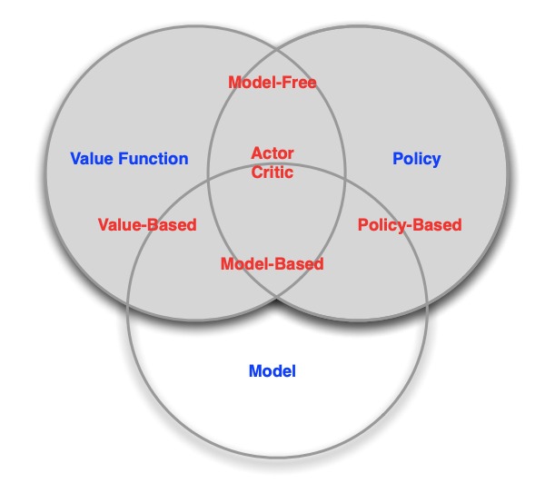
Just as there are many algorithms for regression or classification, there are many reinforcement learning architectures, and new approaches are constantly emerging. Based on which components a reinforcement learning algorithm uses to generate the workflow illustrated in Figure 1, it can be categorized by type.
Figure 2. Variations of Reinforcement Learning
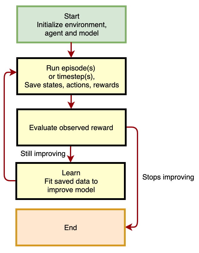
All reinforcement learning variations learn using a similar workflow:
- Initialize the algorithm with naive, typically random, policy parameters.
- Using the policy, take actions, observe states before and after actions, gather experience rewards.
- Fit a model that improves the policy.
- Go to 2) and iterate, collecting more experience with the improved policy, and continuing to improve it.
As we continue to iterate, we improve the algorithm.
Figure 3. Reinforcement Learning Workflow
RL in context
In a previous post we discussed the differences between paradigms of machine learning:
- Supervised learning: Any algorithm that predicts labeled data. Regression predicts a continuous response variable: next quarter’s real GDP growth, next month’s stock return (previous discussion here). Classification predicts a categorical response variable: recession or recovery, next month’s return quintile (previous discussion here).
- Unsupervised learning: Any algorithm that summarizes or learns about unlabeled data, such as clustering or dimensionality reduction.
Any data set is either labeled or unlabeled. So between supervised and unsupervised, that must cover all the bases, right? It’s like those two books, What They Teach You At Harvard Business School and What They Don’t Teach You At Harvard Business School. Between the two of them, they must cover the sum of all human knowledge, right?
Nevertheless, reinforcement learning is considered the third major machine learning paradigm. Consider the Tic-Tac-Toe robot:
- The agent doesn’t have fixed training data. It discovers data via an unsupervised process and learns a policy.
- The rewards can be viewed as labels generated by a supervisor. But rewards aren’t always directly related to one specific prediction or action, or an individual row of data. If the agent shoots a target in Space Invaders, it has to figure out which action or sequence of actions, possibly over many preceding timesteps, contributed to the reward (the credit assignment problem).
- The agent’s interactions with the environment shape that environment, help determine what data the learning algorithm subsequently encounters, and generate a feedback loop. A Space Invaders agent changes the world by shooting targets; a self-driving car doesn’t modify the road, but its actions modify how other vehicles behave, and what environment the algorithm subsequently encounters.
- In supervised learning, the algorithm optimizes model parameters over training data to minimize a loss function, like mean squared error or cross-entropy. In reinforcement learning, the algorithm optimizes model parameters over the state space it encounters, to maximize the expected reward generated by the MDP over time.
In reinforcement learning, we move beyond prediction to control. Reinforcement learning can be viewed as the application of supervised machine learning to a larger problem of optimal control. We apply supervised prediction methods such as classification and regression to choose the best action to take within the action space and learn behavior policies to maximize reward in a complex dynamic environment.
Many disciplines have encountered settings like this and developed methodologies to address them:
- Business/Operations Research: Dynamic pricing of airline seats or other products to maximize profits under changing inventory, production, demand conditions.
- Economics: Optimal Fed interest rate policy to maintain full employment and low inflation in a dynamic economy.
- Engineering: Auto-pilots, spacecraft navigation, robots, and industrial automation.
- Psychology: Stimulus-response, positive and negative reinforcement.
- Neuroscience: The brain’s chemical reward loop, how children learn to walk and talk or catch a ball.
- Mathematics: Control theory, game theory, optimization.
Figure 4. Reinforcement Learning’s Relationships with Science and Engineering Disciplines
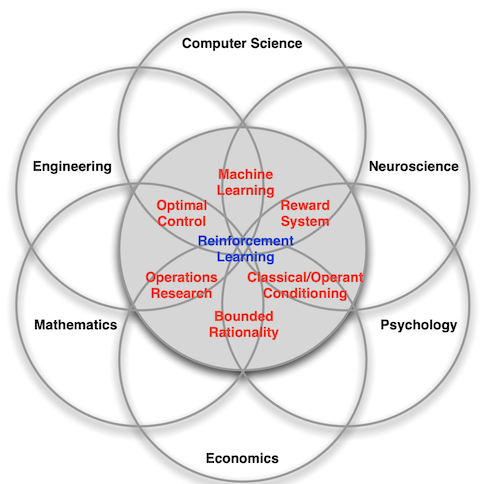
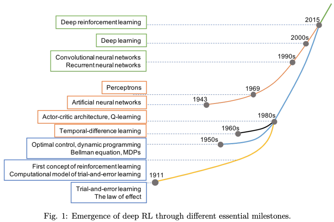
Figure 5. History Milestones in Reinforcement Learning
Deep reinforcement learning for trading applications
Our table lookup is a linear value function approximator. Our linear value function approximator takes a board, represents it as a feature vector (with one one-hot feature for each possible board), and outputs a value that is a linear function of that feature vector, the value score for that board. We dot-multiply the one-hot feature vector by the lookup table values, and we get a linear value function which we use to choose the next move.
We can swap that linear function for a nonlinear function, a neural network. When we do that, we get our first, very crude, deep reinforcement learning algorithm.
Our new deep Q-learning (DQN) algorithm is:
- Initialize our neural network to random weights.
- Play a game with our opponent.
- Append each board we encounter into an n x 9 data array (our predictors) associated with the outcome of the game (our response). Our 9 predictors are the state of each square.
- Fit the neural network to the predictors (vectors representing boards) and responses (win/lose averages) we’ve seen. The neural network predicts the value of each board, instead of a table lookup/linear function.
- Go to 2), gather more data, and continue training to better predict the value of each board.
The more the algorithm plays, the more accurate the function approximator gets, and the better it plays.
This algorithm will learn to play, although it takes a long time to train and makes our initial brute force method even more inefficient. (see code).
But in a nutshell, that is how a self-driving car could work.
- The state is represented by a giant array of inputs from all the onboard cameras and sensors.
- The actions are: turn the steering wheel, accelerate, and brake.
- Positive rewards come from staying on the road and arriving safely at the destination, and negative rewards from breaking traffic laws or colliding.
- The real world provides state transitions.
- And we train a complex neural network to do everything involved in detecting and interpreting all the objects in the environment and navigating from point A to point B.
Table lookup cannot scale to high dimensional or continuous action and state spaces. And a linear function approximator can’t learn nonlinear behavior. With deep neural networks, reinforcement learning algorithms can learn complex emergent behavior.
Simple harmonic motion
In a trading context, reinforcement learning allows us to use a market signal to create a profitable trading strategy.
- You need a better-than-random prediction to trade profitably. The signal can come from regression, predicting a continuous variable; or classification, predicting a discrete variable such as outperform/underperform (binary classification) or deciles (multinomial classification).
- The reward can be the raw return or risk-adjusted return (Sharpe).
- Reinforcement learning allows you to take a signal and learn a good policy (trading strategy) to maximize the reward (return or risk-adjusted return).
Here’s a simple example showing how one can trade using reinforcement learning. This approach is inspired by the paper “Machine Learning For Trading” by Gordon Ritter.
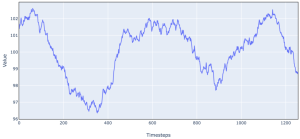
We use simple simulated market data as a stepping stone to more complex trading environments. Let’s create a market price time series as a simple sine wave.
Figure 6. Simulated Stock Price Data (Simple Harmonic Motion)
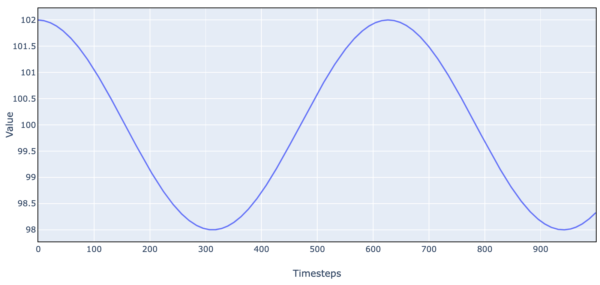
- Initially, we set the price at 102 and price momentum at 0, and 100 as the price ‘anchor’.
- At each timestep, the price accelerates toward 100 by an amount proportional to the distance from 100. If the price is 102:
- the distance from 100 is 2.
- the new price momentum is old momentum – 2 * k.
- the new price is old price + momentum.
We can view this as an extremely simplified value/momentum model. 100 is the intrinsic value the stock tends toward. The farther away from intrinsic value, the stronger the acceleration back toward intrinsic value. And momentum means that if the stock is trending up or down, the trend takes time to be reversed.
To trade this stock, we use the REINFORCE algorithm, which is a Monte Carlo policy gradient-based method. (We can also use Q-learning, but policy gradient seems to train faster/work better.)
We simulate many episodes of 1000 training days, observe the outcomes, and train our policy after each episode.
1) Initialize a neural network to choose actions based on the state.
- 32 inputs: the last 16 market values (as deviations from 100 or intrinsic value), and the last 16 daily changes. (4)
- 2 hidden layers of 16 units.
- 3 outputs of the probabilities of 0, 1, or 2 for short, flat, long respectively (softmax activation, i.e. multinomial classification).
- Initialize neural network θ values at random.
2) Generate one episode trajectory using the current policy. At each timestep:
- Input the current state to the neural network and generate policy probabilities for short/flat/long.
- Sample from the generated probability distribution and take the sampled action.
- Generate a reward based on trading 1 share based on the action taken:
- When our chosen action is 2 (long), the next reward is the change in price at the next timestep.
- When our chosen action is 1 (flat), the next reward is 0.
- When our chosen action is 0 (short), the next reward is the opposite of the change in price at the next timestep.
- Save the observed state, action taken, and reward.
3) At the end of the trajectory, back up and compute a discounted future reward observed at each timestep using the action taken and following the current policy to the end of the episode. (5) Standardize the returns (discounted future rewards) by subtracting the mean and dividing by the standard deviation.
4) Update the policy:
- Compute the gradient vector of each action probability with respect to the policy θ values (the neural network parameters)
- Use the probability gradient to compute the gradient of the expected return overall actions taken with respect to θ. (EV of gradient times return overall probability-weighted actions taken)
- Update each θ by the gradient of expected return w.r.t θ, times a learning rate. In other words, update the policy in the direction that increases the average return overall actions taken as much as possible:
- actions with above-average rewards become more probable
- actions with below-average rewards become less probable
5) return to 2) and iterate until the policy stops improving.
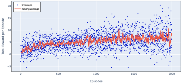
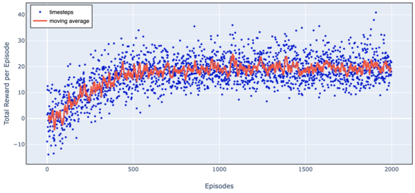
Here is a chart of total reward as we train over 2000 episodes.
Figure 7. Trading Agent Learning Progress (Simple Harmonic Motion)
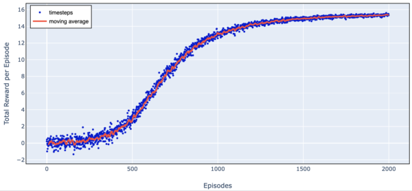
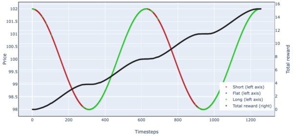
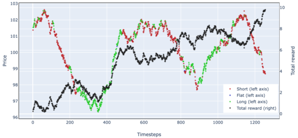
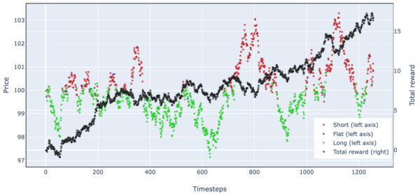
Figure 8. Simulated Stock Trading Results Over One Episode (Simple Harmonic Motion)
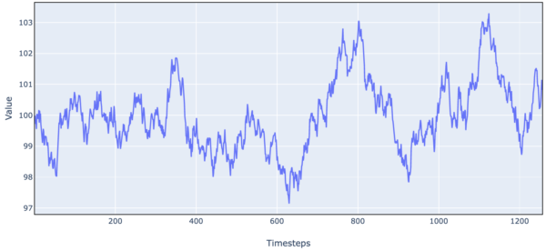
Simple harmonic motion + noise + damping
For a more complex example, we take the simple harmonic motion dynamics and add noise + damping.
Figure 9. Simulated Stock Price Data (Simple Harmonic Motion + Noise + Damping)
Here is an OU process plus noise:
Figure 12. Simulated Stock Price Data (OU Process, Random Walk + Mean Reversion)
But I think this is long enough and sufficient to illustrate the fundamentals of reinforcement learning, and I’ll stop here.
The code for the trading experiments is here.
Advanced technical concepts
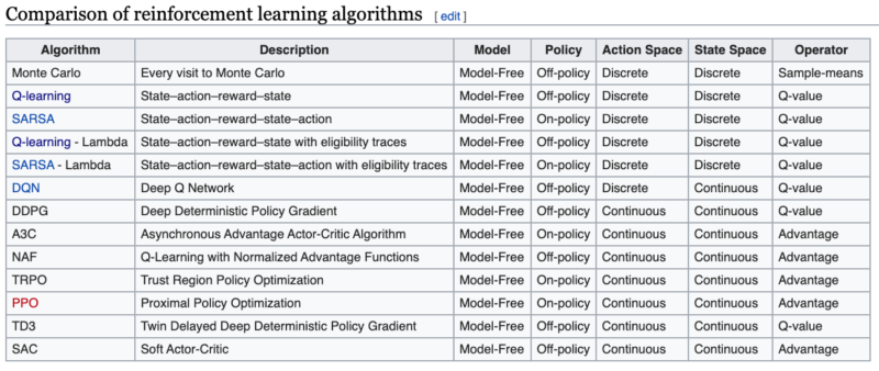
This table from Wikipedia lists some of the variations of reinforcement learning:
Monte Carlo vs. Temporal Difference and the strange-loopy bootstrap
In our policy gradient algorithm:
- We run an episode.
- We back up from the final timestep to the beginning using observed rewards to compute discounted rewards over the full episode.
- We train by ascending the policy gradient that improves standardized rewards.
Sometimes we don’t have short episodes, we have a process that continues forever, or for a very long time. A self-driving car algorithm might have trips with millions of timesteps. An alternative to Monte Carlo training, which runs a full episode and backs up to assign rewards, is temporal difference learning (TD):
- We use a value function that estimates the expected future reward from this state, following the current policy.
- We run one timestep.
- We back up one episode and compute the difference between the expected value we saw at the last timestep and the value after we took this action (the reward from this action, plus the discounted current expected value).
- This improvement is the advantage we got from that action. We train by ascending the θ gradient that improves the probability of the most advantaged actions.
This is a slightly strange magical recursive loop. At the outset, our policy has a random θ. So we are training on the improvement from our fairly random value to the slightly less random value at the next timestep where we know one reward. Nevertheless, as we do this many, many times, the influence of rewards further in the future filters back one step at a time and we bootstrap to a better and better policy.
When we train on the advantage gained using our policy between now and the next step, it’s called TD(0). We can also train on the improvement 2 steps into the future, and that’s TD(1), and we can do TD(2) and so on. If we do TD(∞) we are continuing through the end of the episode, however long it may be, and we are back to Monte Carlo learning.
Finally, there’s a temporal difference algorithm called TD(λ) where we effectively use an exponential moving average of all the TD terms. Setting λ to 0 is effectively TD(0), setting λ to 1 is effectively Monte Carlo, and calibrating λ determines how far into the future we want to peek. With TD(λ), eligibility traces are used to keep track of how much credit to assign to the current action for rewards many steps into the future.
Revisiting value-based v. policy-based methods
- If we do TD learning using only a state-value neural network function approximator, and our policy is to choose the action resulting in the best state-value, this is a Deep Q-Learning Network (DQN).
- If we use only a policy network, this is a Policy Gradient method.
- If we use a value network and a policy network and train the policy function separately so that it improves the value function as much as possible, this is Actor-Critic learning.
The exploration vs. exploitation tradeoff
When we do Q-learning, our policy is to choose the action with the best resulting state-value. However, there is a strong possibility that early in our training one action is always best in some part of the state space. Since we always choose the best action and never try other actions, our training never learns from situations where the other actions may be better.
To avoid this, we perform ε-greedy exploration. Early on, we follow our policy say 60% of the time, and a random action 40% of the time. This allows the algorithm to experience the whole state/action space. 40% is the ε parameter. In practice since our policy network is random at the outset, we typically start with ε at 100% and gradually reduce it to a very small value.
On-policy vs. off-policy learning
ε-greedy algorithms are ‘off-policy’ learning since they sometimes act differently from the policy and train on the resulting outcomes, in contrast to algorithms which only take ‘on-policy’ actions. Policy gradient algorithms sample actions from a probability distribution. Bad actions never have a strictly zero probability, they just get less likely over time. So sampling implicitly trades off an exploration of new actions, vs. exploitation of the best actions.
TRPO and PPO, or how to avoid falling off a cliff
Finally, we have noticed that sometimes training will fall off a cliff. Through the extreme nonlinearity of neural networks, a small gradient descent update may generate a large change in policy outcomes. Sometimes the policy is much worse and the training optimization has trouble climbing back up, like falling into a crevasse on the way up Mount Everest. One might avoid that with very small steps, i.e. a small learning rate, but then training takes forever. Two popular variations that address this issue are Trust Region Policy Optimization (TRPO) and Proximal Policy Optimization (PPO). Essentially they avoid or penalize updates that change the output policy too much in one update.
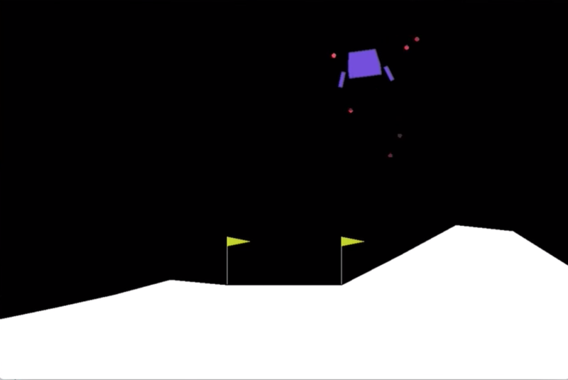
I experimented with a few algorithms in the OpenAI gym, using Cartpole and Lunar Lander here. This is a good way to get started learning about RL, along with more resources listed below.
Takeaways
Like the man in the Molière play who discovers he’s been speaking in prose his whole life, you may have been doing reinforcement learning and optimal control your whole life without realizing it.
Reinforcement learning is an important paradigm in machine learning. It can bridge a gap between predicting and doing, between description and prescription. And many markets and economic processes can be impacted by adaptive intelligent agents.
In quant investing, sometimes one finds that a modest predictive R-squared, or a modest change in behavior, avoids the actions with worst outcomes, and leads to a large improvement in returns. At other times, one finds that a significant improvement R-squared offers no investment performance improvement.
Why is that? Hypothetically, suppose you have a stock that in the long run yields a 5% annualized return. And the single best day each year is up 5%.
Suppose you discover a classifier or regression that always gets that one day right, and is no better than random the rest of the time. With a fraction of a percent increase in accuracy or R-squared you almost doubled your expected return.
Suppose you can also get a perfect prediction on all the days when the daily return is close to 0. On those days, it doesn’t matter if you are long or not. Under a perverse scenario, you could improve your forecast on every one of those days, and improve your predictive R-squared or classifier accuracy a lot. But if you do that, it won’t improve your performance. And if you then miss that one good trade, you worsen the investment outcome, possibly even while improving R-squared.
Prediction and control are two different objectives. If you have a perfect prediction, then you always choose the correct action, and you have perfect control. But you only need a good enough prediction to select the correct action. Beyond that, any further accuracy is superfluous. And you can sometimes select the correct action at the most critical time and can get pretty good control outcomes, with only a modest predictive signal. (6)
In the spirit of deep learning, reinforcement learning trains a complex neural network directly on the reward. Training directly on the reward to choose actions will tend to focus the algorithm on the situations where the choice of action makes the biggest difference. If you train for prediction first, and then use prediction for control, the training values any improvement in prediction equally, even if it doesn’t improve control. In deep learning, we don’t necessarily break down a complex engineering problem into more tractable components. Instead, we ask what complex model would be able to solve a complex problem, and train the model end-to-end for a long time on big data. Often, this yields emergent behavior and unreasonably effective models.
The link between statistical prediction metrics and real-world performance can be elusive. But in general, reinforcement learning will learn to use whatever forecasting edge it has, to generate a maximum reward in a dynamic environment.
How is reinforcement learning different from backtesting? Backtesting exhaustively searches a parameter space for a parameter vector that obtains the best out-of-sample performance. When we use reinforcement learning with a function approximator and gradient descent, we can use much more complex models where there are too many parameter combinations to backtest, but still efficiently explore the search space and possibly obtain a better result. Training complex models end-to-end simultaneously for prediction and control can result in complex emergent behavior that displays almost human-like intelligence, and adaptive behavior.
There is a parallel between reinforcement learning and the adaptive market hypothesis of Andrew Lo. Markets may not be perfectly efficient at all times, but they tend to move in that direction via an evolutionary learning process based on experience.
JPMorgan and others have reportedly implemented reinforcement learning to trade in the real world, see for instance this paper and (more readable) article. In another example, Igor Halperin used reinforcement learning to successfully model the return from options trading without any Black-Scholes formula or assumptions about log-normality, slippage, etc.
Thesis:
- Reinforcement learning can learn complex economic decision-making in many cases better than humans.
- Reinforcement learning can develop concepts like how to maximize risk-reward without knowing the CAPM or Black-Scholes.
- Economic and finance theories can be tested empirically in silico by creating multi-agent reinforcement learning experiments where we just tell agents to maximize a reward and see what behaviors they learn.
- Therefore, we don’t need economists to develop fancy models, we don’t need traders to execute trading strategies, and intelligent agents will take over real-world economic decisionmaking. Agents will move from trading algos to setting prices on Uber and Amazon, to controlling the traffic lights, congestion pricing, and information flow in a transportation network to keep traffic moving.
Antithesis:
- Reinforcement learning is very data-hungry or sample-inefficient, more suited to intraday trading, not lifetime 20-punchcard type problems.
- High model complexity makes interpretability challenging.
- It doesn’t always work. Reinforcement learning can get stuck at local optima or fall off a cliff. You have to take care to not just train on recent experience but also important but rare cases, the way pilots train for equipment failure and upset recovery.
- AI algorithms can be exploited. An adversarial sticker can make image recognition think a banana is a toaster or an adversarial temporary tattoo can defeat facial recognition. Google’s traffic algorithm can be gamed. Trading is an adversarial game against highly adaptive competitors. If a market maker algorithm trades on patterns, adversarial algorithms can learn to manipulate it, paint the tape to make it do bad trades.
Synthesis: It’s hard to tell what will happen but it will certainly be interesting.
When many agents interact in a market and try to learn an optimal policy at the same time, the environment becomes radically non-stationary. If a self-driving car crashes on an empty track in a single-agent environment, it has to learn which of its actions caused the crash. But in the multi-agent setting, if it crashes into another car, it has to model why the other car did what it did and adjust behavior accordingly. With multiple agents interacting, they have to ask themselves not only how much reward to attribute to which past actions they took, but how much credit or blame to attribute to each agent.
You get feedback loops and unexpected emergent behavior. In real-world economics or trading settings, maybe agents adapt to each other and arrive at a new, more efficient price equilibrium. Maybe they create extreme algorithm-induced oscillations between multiple equilibria. Maybe they learn to collude? We don’t know. It depends on the market structure, the diversity of the robot population, etc. What we do know is it becomes an NP-hard problem to find a multi-agent policy with optimal outcomes.
I’m not sure self-driving vehicles on the streets of New York or New Delhi are likely in the near future, without protected rights of way for self-driving vehicles and strong enforcement. If pedestrians know that the self-driving car is always going to stop for them no matter what, they will learn to just cross at the red light, never mind traffic. They can even wear a stop sign on a T-shirt. It’s not a question of how good the self-driving technology is, it’s a question of game theory. Knowing that the other driver is a fallible fellow human, who may be angry and honk and give you the finger, and at worst may be on a cell phone and not even see you, just leads to different outcomes.
Reinforcement learning and intelligent agents may offer economics a path out of the DSGE/microfoundations conundrum. Would you rather have a model that empirically works pretty well in the current real-world regime; or a less accurate model based on a strong theoretical foundation and therefore more robust to regime shifts?
By complexifying the representative agent, maybe you get more predictive or at least more interesting micro-founded models. You can ask questions like, what conditions are necessary and sufficient for smart Prisoners Dilemma agents to move from the naive Nash equilibrium where they are better off always defecting, to a meta-Nash equilibrium where every agent has no incentive to deviate from the policy of always cooperating.
Economics and finance involve thinking about how systems of interacting, constantly adapting, intelligent agents behave. It seems likely more of them will be non-human, and the whole world will be a lab.
“We shape our tools and thereafter our tools shape us” – John Culkin
Further reading
Papers and blog posts:
- Csaba Szepesvári, Algorithms for Reinforcement Learning
- Andrej Karpathy: Deep Reinforcement Learning: Pong from Pixels
- OpenAI: Key Papers in Deep RL
- Yuxi Li, Deep Reinforcement Learning
- Thomas G. Fischer, Reinforcement Learning in Financial Markets – A Survey
- Gordon Ritter, Machine Learning for Trading
- Heaton, J.B. and Polson, Nick and Witte, Jan, Deep Learning for Finance: Deep Portfolios
- Kaiqing Zhang, Zhuoran Yang, Tamer Başar, Multi-Agent Reinforcement Learning: A Selective Overview of Theories and Algorithms
- Afshin OroojlooyJadid and Davood Hajinezhad, A Review of Cooperative Multi-Agent Deep Reinforcement Learning
- Alex Irpan, Deep Reinforcement Learning Doesn’t Work Yet
- Python implementations of RL algorithms: Lilian Weng; Denny Britz; Arthur Juliani
- Contests: Google Research Football; Pommerman; MineRL
Books:
- Reinforcement Learning: An Introduction, Richard S. Sutton and Andrew G. Barto
- Foundations of Deep Reinforcement Learning: Theory and Practice in Python, Laura Graesser, Wah Loon Keng
- Deep Learning, Ian Goodfellow and Yoshua Bengio and Aaron Courville
- Artificial Intelligence: A Modern Approach, Stuart Russell, Peter Norvig
Courses:

References[+]
| ↑1 | Even if they are isomorphic to boards it has seen. There are really only 3 starting moves, board center, corner, center side. Flipping or rotating the board shouldn’t change the value of a position or how to play it. |
|---|---|
| ↑2 | Or ot, the observable part of the state, in the event the state is not fully observable, and there is some hidden state that determines the evolution of the game, such as face-down cards. |
| ↑3 | For instance, instead of a table with all possible Tic-Tac-Toe boards we could use a table mapping (board, action) pairs to values. Then we wouldn’t be modeling internally what happens after a move, i.e. several (board, action) pairs arrive at the same board. We would just evaluate state, action pairs directly without any internal model. That would work pretty much the same, it would just be a bigger table and take longer to train. |
| ↑4 | For our simple harmonic motion with no noise, one input of the last change is sufficient. But a more complex model with 16 days of levels and changes can be applied to a more complex example. |
| ↑5 | In this simple model, we can use a large discount because each action only influences the next trading day. In a more complex environment where the current action can impact rewards far in the future, we would want to take those rewards into account, and we would use a smaller discount. |
| ↑6 | The context here is a price-taking trading algorithm too small to influence the overall market. Of course, an algorithm playing poker or Atari or Google Football tries its utmost to influence the course of the game to its advantage. The most important difference between prediction and control is how the algorithm alters the dynamics of the game, and the resulting feedback loop. A reinforcement learning trading algorithm will tend to reinforce any actions that earn a reward, including influencing the market, painting the tape, or colluding with other market participants. |
About the Author: Druce Vertes
—
Important Disclosures
For informational and educational purposes only and should not be construed as specific investment, accounting, legal, or tax advice. Certain information is deemed to be reliable, but its accuracy and completeness cannot be guaranteed. Third party information may become outdated or otherwise superseded without notice. Neither the Securities and Exchange Commission (SEC) nor any other federal or state agency has approved, determined the accuracy, or confirmed the adequacy of this article.
The views and opinions expressed herein are those of the author and do not necessarily reflect the views of Alpha Architect, its affiliates or its employees. Our full disclosures are available here. Definitions of common statistics used in our analysis are available here (towards the bottom).
Join thousands of other readers and subscribe to our blog.