Benjamin Graham, often considered a strong candidate for “the father of quantitative value investing“, developed an investment strategy that involved purchasing securities for less than their “current-asset value”, “a rough index of the liquidating value”. We uncovered ten research papers that examined the returns achieved by investing in such securities which were conducted over a number of decades and across various geographies. In general, the research found that the strategy generated a remarkable level of outperformance. Based on what we know about the “publication bias,” perhaps this is not too surprising.
However, our objective in reviewing this collective research was not to identify if the Graham “Net-net” strategy works from a historical perspective, instead, we seek to answer the following question, “Could the returns reported in the research have been achieved by an investor in practice?”
To meet this objective, we developed a methodology to analyze the evidence and determine its reliability. Subsequently, we found that each of the studies suffered, or may have potentially suffered, from a number of biases that adversely impacted the reliability of the results contained therein. We, therefore, concluded that, in essence, a practitioner could not have achieved the returns reported in the research. Lastly, we briefly discussed the implications of our findings for practitioners of the investment strategy, as well as for evidence-based investors at large.
The History of the Net-Net Value Investing Strategy
In 1934, between two world wars and in the midst of the great depression came the publication of Security Analysis by Benjamin Graham and David Dodd, an investment classic.
“A classic is something that everybody wants to have read and nobody wants to read.”
attributed to Mark Twain
Within the weighty tome Graham details an investment strategy that involves purchasing stocks for less than their “current-asset value”, “a rough index of the liquidating value”.(1) In turn, the “current-asset value of a stock consists of the current assets alone, minus all liabilities and claims ahead of the issue. It excludes not only the intangible assets but the fixed and miscellaneous assets as well.”(2) Colloquially, such firms are referred to as “net nets” because their market capitalization is “net” of the “net current asset value”.(3)
For context it is worth noting that the Dow Jones Industrial Average (DJIA) reached 381.17 on September 3, 1929 and bottomed at 41.22 on July 8, 1932 – an 89.2% drawdown!(4) One can only marvel at the intestinal fortitude demonstrated by implementing any stock investment strategy in the face of such capital destruction.
Furthermore, with the behaviour of the market such as it was in the lead up to the publication of Security Analysis, one wonders how Graham’s faith was maintained in the behaviour of market participants, given the ultimate reliance on market participants to achieve the desired capital appreciation.
“Successful investing is having everyone agree with you… later”
Jim Grant
Graham is often considered to be the father of value investing. However, despite such reverence, his strategy of purchasing securities trading at less than their Net Current Asset Value (NCAV) has been the focus of relatively limited research. In our quest for research examining the returns achieved by purchasing such securities, we uncovered ten studies that were conducted by academics and practitioners alike.
The Objective
Our analysis was focussed on answering one primary question:
Could the returns reported in the research have been achieved by an investor in practice?
At first glance it seems an almost preposterous research endeavour; why examine something that is seemingly self-evident? Well, the returns reported in the majority of the research revealed an outperformance of such magnitude that our inherent skepticism stirred us into a forensic examination.
“[I]n theory there is no difference between theory and practice, while in practice there is”
Benjamin Brewster (often attributed to Yogi Berra)
The Methodology
In order to meet our research objective and answer the question, “Could the returns reported in the research have been achieved by an investor in practice?”, we systematically and objectively analysed each study in its own right. Accordingly, we analysed a cross-section of items in each of the studies including, but not limited to, the: valuation metric, weighting method, purchase/rebalancing rules, portfolio formation methodology and holding period(s). With regard to reliability specifically, we analysed the studies for: survivorship bias, look-ahead bias, sample size issues, potential for human error, publication credibility, time period bias, data source reliability, minimum market capitalization requirements, return calculation methodology and errors generally.
To enhance understanding we provide additional detail pertaining to certain items below:
Time period bias
In general, the longer the test period the more reliable the results, the shorter the test period the less reliable the results. That said, where individual studies are deemed reliable, but for the time period utilized, we could potentially marry them to other such studies and aggregate the results in an attempt to circumvent the time period bias.
According to commentary and research published in “What Works on Wall Street (Fourth Edition)” by James O’Shaughnessy investing the lowest (i.e. cheapest) decile of stocks sorted by price to book has produced material outperformance for periods as long as 18 years. However, over even longer periods that relationship has not held. Ideally then, we would want multi-decade examination periods to be employed. (here is a simulation study on value portfolios to add additional context)
We used the following ranges to determine the presence of time period bias:
- < 10 years; inadequate/unreliable
- 11 to 20 years; somewhat reliable
- 20 years; more reliable
- 40 years; most reliable
Data source reliability
A reliable and reputable data source is a necessity when conducting empirical research. Seemingly, the utilization of the CRSP/Compustat data base covering US-listed securities from 1926, the gold standard in stock research, would circumvent any concerns when examining US listed securities. Unfortunately, even this database has had concerns raised over its reliability in a highly recommended article titled “The Myth of 1926: How Much Do We Know About Long-Term Returns on U.S. Stocks?” by Edward F McQuarrie.(5) McQuarrie finds that, in essence, 1973 onwards represents the point at which data contained within the CRSP/Compustat data base is most reliable. However, in a final twist James O’Shaughnessy states in “What Works on Wall Street (Fourth Edition)” that “[c]ompustat also added many small stocks to its dataset in the late 1970s that could have caused an upward bias to result, since many of the stocks added were added because they had been successful.”
Consequently, if even the leading database for empirical research into stocks has question marks over its reliability, we would be wise to assume that other databases may also suffer from some form of bias or contain errors of some degree.
Minimum market capitalization requirement
For an investment strategy to be effective, it must be tradable in practice. However, some studies do not mandate a minimum market capitalization requirement for the stocks contained in the investment universe under examination. Consequently, the results in such studies can be unduly influenced by stocks that are, in practice, virtually untradeable, even when attempting to deploy relatively modest amounts of capital.
To be clear, we do not refer to mere micro capitalization stocks, despite their identification as a major source of the proliferation of “anomalies” identified by academics.(6) In fact, we are not even concerned with stocks close to the upper bound of “nano capitalization” classification per se.(7) Rather, our concern lies with the very smallest stocks that trade infrequently and at a very low “dollar” volume.
We have seen empirical evidence where the smallest decile of stocks was reported to have generated a Compound Annual Growth Rate (CAGR) of 84%!(8) Of course, the driver of those returns were almost certainly stocks that were uninvestable in reality. We explore this issue further by referring once again to “What Works on Wall Street (Fourth Edition)” by James O’Shaughnessy. O’Shaughnessy found that between 1964 and 2009 stocks with a market capitalization less than a deflated USD 25 million (2009 dollars) generated a CAGR of 63.2%!(9) However, “when you require that all stocks have share prices of greater than $1, have no missing return data, and have limited the monthly return on any security to 2,000 percent per month” the CAGR fell to 18.2%. Furthermore, when the analysis was extended to 1926 he found that the CAGR fell to 15%. And finally, “[w]hen you look at the results for investable microcap names, those with market capitalizations between a deflated $50 million and a deflated $250 million, you see that most of the return for tiny stocks disappears.”
Incorporating the principle identified above, where research contains (or may contain) stocks that are (or likely to be) untradeable we may refer to it as suffering from “uninvestable stock bias”.
Return calculation methodology
To achieve our objective of answering the question, “Could the returns reported in the research have been achieved by an investor in practice?”, the answer was reliant on the return methodology adopted to quantify the reported returns.
What follows is a list of the various terminology used to describe the returns in the studies examined: annual geometric mean return, mean returns, abnormal performance, abnormal return, average raw buy-and-hold, average market-adjusted buy-and-hold, abnormal buy-and-hold performance, average return p.a., market return, raw returns, market index returns, buy-and-hold raw return, market-adjusted return, average raw return, average return, compound annual growth rate, cumulative raw return, excess return, percentage of positive excess return, cumulative excess return, simple average, and annualized return!
While the jargon is mind-boggling, in general, the returns reported in the research generally refer to two simple return calculation methodologies: the arithmetic mean and/or the geometric mean.
In a dependant return series that exhibits volatility (like stock returns) the arithmetic mean will, as a matter of mathematical law, overstate returns relative to the geometric mean.(10)
For ease of reference, where returns have been calculated using the arithmetic mean we may simply refer to the research as suffering from “inflated return bias.”
For clarity, it should be noted that the geometric mean, when calculated for annual periods is also often referred to as the Compound Annual Growth Rate (CAGR) or the “annualized” return. The geometric mean return represents the actual return potentially achievable by an investor in practice, and therefore it is the sought-after measure when quantifying investment returns.
Given the importance of the return calculation methodology a few rudimentary examples are worthwhile. Firstly, let us assume an investor starts with $100 and they incur a 60% loss after 1 year resulting in a portfolio value of $40 ($100 * (1 – 60%)). Then, in year 2 they generate a 100% gain resulting in a final portfolio value of $80 (40 * (1+100%)). The arithmetic average return in this case would be 20% ((-60% + 100%) / 2)! Clearly, the result is nonsensical to an investor in practice. In contrast, the geometric mean would reflect practitioner reality and yield a result of -10.56% (80/100^(1/2)-1).
Another theoretically extreme example is provided in the table below:
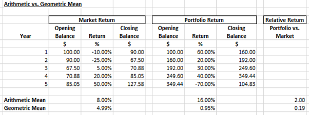
The results are hypothetical results and are NOT an indicator of future results and do NOT represent returns that any investor actually attained. Indexes are unmanaged, do not reflect management or trading fees, and one cannot invest directly in an index.
Remarkably, it is theoretically possible to achieve an arithmetic mean twice that of the market (16.00% vs 8.00%; 2x); and simultaneously attain only a fraction of that return based on the geometric mean (4.99% vs 0.95%; 0.19x).
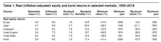
Finally, we provide a practical and wholly independent example to illustrate the misleading nature of an arithmetic mean when dealing with investment returns. Accordingly, we reproduce below Table 1 from the “Summary Edition Credit Suisse Global Investment Returns Yearbook 2019”:
The results are hypothetical results and are NOT an indicator of future results and do NOT represent returns that any investor actually attained. Indexes are unmanaged, do not reflect management or trading fees, and one cannot invest directly in an index.
There is a material difference between the arithmetic and geometric mean achieved for all equity markets examined. For Japan, the arithmetic mean is more than double the geometric mean!
Notwithstanding that discussed above, one may still be tempted to use the arithmetic mean as a guidepost to estimate the more practically meaningful geometric mean; we would caution against such an endeavour. In addition to the mathematical pitfalls illustrated in our examples above, psychologically speaking, such thinking may be driven, in part, by confirmation bias (“net nets outperform!”) and sunk cost fallacy (i.e. having put in the time and effort to read a study one may want to walk away “knowing something definitive”). In addition, statistically, as the number of holdings in a portfolio falls (an issue when examining the relatively small universe of firms trading below NCAV) the volatility of that portfolio may increase thereby leading to a greater potential divergence between the geometric and arithmetic mean. How portfolio volatility changes with the number of holdings in a portfolio was examined, for example, by Elton and Gruber in “Risk Reduction and Portfolio Size: An Analytical Solution” and by Alpha Architect here and here.(11)
So, mathematically, psychologically and statistically attempting to estimate the geometric mean is precarious and even more speculative than it may initially appear.
“The first principle is that you must not fool yourself and you are the easiest person to fool.”
Richard P. Feynman
This leads us to an obvious question, “Why would you use an arithmetic mean to calculate stock returns?”. Indeed, when it first dawned on us that such a methodology was used to quantify stock returns, we were left utterly dumbfounded. We asked finance academics why they utilize the arithmetic mean, and the primary reasons given were that it is:
- Required for the statistical methods applied in academic research e.g. regression analysis
- Used to calculate risk measures e.g. Sharpe ratio, standard deviation etc.
- Used to circumvent the effect of the start and end date which may unduly influence the returns
While the above serves a purpose in academic research it does little for an investment practitioner trying to determine how much they can earn on their capital in reality.(12) While on occasion academic research does contain the geometric mean return (i.e. CAGR) it is not, in our experience, a common occurrence.(13) Indeed, most academic finance research appears to be conducted using arithmetic mean returns. Simply including the CAGR alongside the arithmetic average within academic research would greatly enhance its utility to the practitioner community, and we hope the measure is increasingly adopted. That said, it is our understanding that the academic community rejected the notion of “maximum drawdown” as a measure of “risk”, despite it being arguably the most important risk-related metric for a practitioner. (14) Consequently, the adoption of seemingly “common sense” measures may not be as inevitable as one would hope. Indeed, there appears to be a significant gap between the ivory tower and practitioner land, consequently, we are probably all the poorer as a result.
While our overall methodology used to examine the various studies may seem onerous, we believe it was required as all too often we have seen the cognitively deficient assertion that “all the evidence about “x” says “y” without any thorough examination of underlying evidence, in and of itself. It goes without saying, no matter the quantum of studies showing the same or similar results they remain collectively worthless if they each contain material methodological flaws – they ought to be dismissed rather than “anchored” to in the mistaken belief that they possess some utility.(15)
It is often said “I’ve never seen a bad back test”. We think it prudent to amend that quote to, “I’ve never seen bad back test results!”.
The Evidence
The table below lists the research papers examined along with their key parameters and stipulated returns:
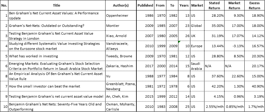
The results are hypothetical results and are NOT an indicator of future results and do NOT represent returns that any investor actually attained. Indexes are unmanaged, do not reflect management or trading fees, and one cannot invest directly in an index.
A summary analysis of each study follows. We encourage readers to refer to the corresponding detailed analysis as well as the original research paper as nuance and clarity may be lost in the pursuit of relative brevity.
The Analysis on Graham’s Value Strategy
Ben Graham’s Net Current Asset Values: A Performance Update
“Ben Graham’s Net Current Asset Values: A Performance Update” by Henry R. Oppenheimer was published in the Financial Analysts Journal (1986). The study examined the performance of securities that were trading at no more than two-thirds of their NCAV during the 13 year period from 1970-82 period in the US.
Results and Analysis
Table IV from the study is reproduced below:
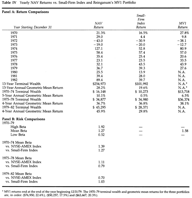
The results are hypothetical results and are NOT an indicator of future results and do NOT represent returns that any investor actually attained. Indexes are unmanaged, do not reflect management or trading fees, and one cannot invest directly in an index.
Below we have adapted the data from Table IV and looked at the performance in both absolute and relative terms to the S&P 500 Total Return (TR, i.e. including dividends):
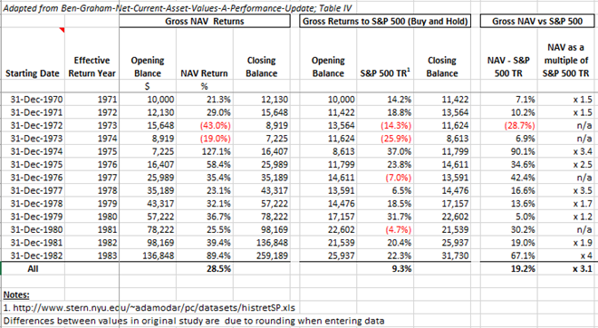
The results are hypothetical results and are NOT an indicator of future results and do NOT represent returns that any investor actually attained. Indexes are unmanaged, do not reflect management or trading fees, and one cannot invest directly in an index.
Gross returns: CAGR of 28.5% (with rounding impacting our calculations) vs 9.3% for the S&P 500 TR; an absolute outperformance of 19.2% and a multiple of 3.1 relative to the S&P 500 TR.
We then simulated reality by adding commissions and taxes to quantify the potential “net returns”. Commissions of 5% (2.5% to buy 2.5% to sell) were incorporated and we utilised the capital gains taxes rates of the corresponding years in the study.(16) Where applicable, we adjusted for tax loss carry forward and assumed our hypothetical investor resided in the US and sat in the highest marginal tax bracket but held on long enough to be eligible for the long-term capital gains tax rates. In contrast, we assumed an investor in the S&P 500 bought and held, never realizing their gains (and for simplicity we did not adjust their dividends for tax).
Net returns (i.e. including commissions and taxes): CAGR of 18.9% vs 9.3% for the S&P 500 TR; an absolute outperformance of 9.6% and a multiple of approximately 2.0 relative to the S&P 500 TR.
Earnings and Dividends
Table V from the study is reproduced below:
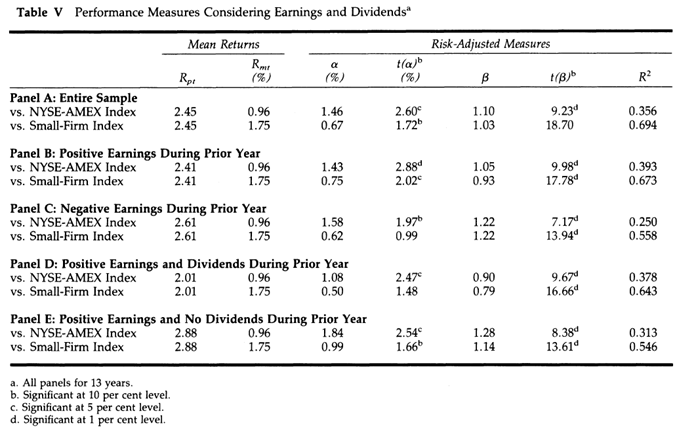
Reconciliation work carried out in our detailed analysis led to the determination that table V reports arithmetic mean returns and therefore suffers from inflated return bias. Nonetheless, we proceed with our examination.
Dividends
When it comes to dividends the spread between “Positive Earnings and Dividends” (Panel D) and Positive Earnings and No Dividends (Panel E) is stark. No economic rationale comes to mind for why a net net paying dividends would underperform one that does not pay dividends.
However, as it often is, the devil is in the details, which appear to have gone unnoticed since publication in 1986:
Note 9 (p. 47) specifies the following:
“all comparisons with the exchange benchmarks returns without dividends are used for both the security return and the benchmark return.”
That is to say, to our understanding, the dividends have been excluded in the returns displayed in Table V (among others), and therefore the returns have been artificially reduced by the amount of the dividend paid out. On that basis it is not at all unexpected that the dividend payers would seemingly underperform their non-dividend paying counterparts.
In light of the above, we are of the opinion that no reliable conclusion can be drawn in relation to the impact of dividends on the returns of “net nets” based on this study.
Earnings
The author sees the differential between “Positive Earnings” (Panel B) and “Negative Earnings” (Panel C) as marginal. The author concludes that “No clear-cut pattern emerges from an examination of these panels. If anything, firms operating at a loss seem to have slightly higher returns and risk than firms with positive earnings.”
It is possible (probable in our view) that “positive earners” had a greater propensity to pay dividends. Therefore, if those dividends were not included in the measurement of their returns they would be artificially reduced. Of course, it is also possible (albeit unlikely in our view) that “negative earners” paid the greater share of dividends subsequently understating their returns. Irrespective, we are of the opinion that no reliable conclusion can be drawn in relation to the impact of earnings on the return of “net-nets” based on this study.
Minimum market capitalization requirement
No minimum market capitalization cut-off for the securities examined in this study was mandated. Furthermore, we note that the reported median market capitalization of securities in the portfolios examined was 4.1m. That is to say, half the firms examined had a market capitalization equal to or below 4.1m which is particularly small, even by today’s inflation-adjusted standards. In light of the foregoing, it is highly probable that a considerable number of firms included in the study were, in effect, uninvestable.
Conclusion on “Ben Graham’s Net Current Asset Values: A Performance Update”
While compounded gross returns were provided in some instances, certain sub-strategies were measured using the arithmetic mean returns, and therefore they suffered from inflated return bias. In addition, the study utilized data that excluded dividends thereby compromising the reliability of a number of conclusions reached therein.(17) Critically, it is highly probable that the reported returns were impacted by uninvestable stock bias.
Detailed analysis: An Analysis of “Benjamin Graham’s Net Current Asset Values: A Performance Update” (also available on Alpha Architect here).
Graham’s Net-Nets: Outdated or Outstanding?
“Graham’s Net-Nets: Outdated or Outstanding?” published in “Value Investing: Tools and Techniques for Intelligent Investment” by James Montier (2009) examined the performance of securities that were trading at no more than two-thirds of their “net current assets” during the 23 year period from 1985-2007 globally and regionally (namely, in the US, Europe, and Japan).
Results and Analysis
“An equally weighted basket of net-nets generated an average return above 35% p.a. versus a market return of 17% p.a.”
“Not only does a net-net strategy work at the global level, but it also works within regions (albeit to varying degrees). For instance, net-nets outperformed the market by 18%, 15%, and 6% in the USA, Japan and Europe, respectively.”
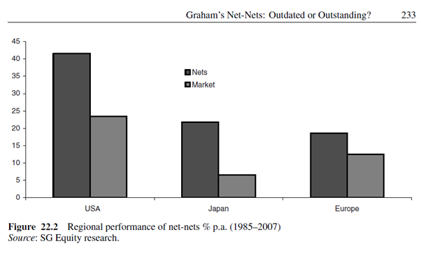
We summarise the results in the table below (some of which were gleaned from Figure 22.2):
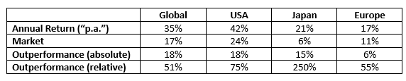
The results are hypothetical results and are NOT an indicator of future results and do NOT represent returns that any investor actually attained. Indexes are unmanaged, do not reflect management or trading fees, and one cannot invest directly in an index.
It should be noted that no detail pertaining to the methodology and data source used to undertake study was disclosed.
In our detailed analysis, we reconciled the returns to references made to the Oppenheimer study. We identified, “with a strong likelihood, that the author has calculated the arithmetic mean return”, and consequently that the reported returns were overstated.
We also stated that “… a cursory glance at Figure 22.2 illustrates returns of 24% p.a. to the “USA Market” from 1985-2007; this also indicates an arithmetic mean has been used because, to our knowledge, the US market simply did not achieve a compound annual growth rate of 24% from 1985 to 2007!”. No information was disclosed with regard to the index used to represent the “USA Market”. However, it should be noted that the arithmetic mean return for the S&P500 (including dividends) from 1985 to 2007 was 13.65%; nowhere near the 24% graphically represented!(18)
Conclusion on “Graham’s Net-Nets: Outdated or Outstanding?”
The returns reported in “Graham’s Net-Nets: Outdated or Outstanding?” were not compounded returns (i.e. geometric mean returns). Whatever the return calculation methodology adopted, it appears that even their graphical representation is erroneous. Consequently, in our opinion, no credibility whatsoever ought to be attributed to the returns reported in the study.
Detailed analysis: An Analysis of “Graham’s Net-Nets: Outdated or Outstanding?” (also available on Alpha Architect here).
Testing Benjamin Graham’s Net Current Asset Value Strategy in London
The objective of the paper, “Testing Benjamin Graham’s Net Current Asset Value Strategy in London”, was to examine the performance of securities that were trading at greater than 1.5 times the Net Current Asset Value (NCAV)/Market Value (MV) (i.e. less than 2/3 of NCAV) during the 26 year period from 1980 to 2005 on the London Stock Exchange.
Results and Analysis
Table 2 from the study is reproduced below:
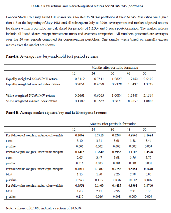
The study reported an average raw buy and hold return of 31.19% to the NCAV portfolios 12 months after formation! What exactly are “average raw returns” and are these returns truly reflective of a practitioner’s reality? Significantly, the “Average raw returns” are calculated as the arithmetic mean of returns; consequently, the study suffered from inflated return bias.(19)
Furthermore, the authors did not mandate a minimum market capitalization cut off for the securities they examined, and as a result they included even the very smallest firms in the market.
They state “…stocks are allocated to an NCAV/MV portfolio if their ratio is higher than 1.5. The numbers shown are the percentage of the average NCAV/MV portfolio falling into each size decile.… nearly 79 percent number of companies are very small (belong to size 1 and size 2)”. Table 6, which confirms the aforementioned is reproduced below:

The smallest decile of the market is where 63.23% of the investment candidates were identified, and it is in this decile where the greatest trading constraints are likely to be faced. From table 2 we note that “value weighting” the NCAV/MV portfolio resulted in a 4.58% (31.19% – 26.61%) reduction in the “average raw buy-and-hold” return for portfolios held for 12 months; this implies that the smallest stocks disproportionately contributed to the reported outperformance.
Therefore, not only were the reported “average raw returns” unattainable in practice, they were also highly likely to have been afflicted by uninvestable stock bias.
Conclusion on “Testing Benjamin Graham’s Net Current Asset Value Strategy in London”
The study suffered from inflated return bias and is highly likely to have also suffered from uninvestable stock bias thereby rendering the reported returns unattainable in reality.
Detailed analysis: An Analysis of “Testing Benjamin Graham’s Net Current Asset Value Strategy in London” (also available on Alpha Architect here).
Studying Different Systematic Value Investing Strategies on the Eurozone Market
In 2010 investment practitioners Philip Vanstraceele and Luc Allaeys published a research paper titled “Studying Different Systematic Value Investing Strategies on the Eurozone Market” which examined the performance of stocks in the “Eurozone” identified by a NCAV screen during the 10 year period from 1999 to 2009.
The paper claimed, “In our methodology the NCAV-ratio should be greater than 1,33, and we define the ratio as Net Current Assets Value / Market Value. This ratio is used to find companies that are trading below their net current assets value.”
For clarity, it should be noted that a ratio of 1.33 of Net Current Asset Value/Market Value equals 75% of NCAV.
Upon further analysis the claim appeared to be spurious in light of the sheer number of firms they reported to have tested at various market capitalization cuts offs. And indeed, upon further investigation our strong suspicion was confirmed.(20)
In fact, what was actually tested were those firms that traded at the highest relative “ratio of Net Current Assets Value / Market Value” (MV), not what was specified in the methodology of the study. Having established that we can proceed with a review of the returns achieved. The measure of relative cheapness may at least provide us with an insight as to the ability of the NCAV/MV metric to sort “winners” from “losers”.
Results and Analysis
Significantly, the authors examined the returns by calculating the CAGR.
We have restated the returns as reported in the study with regard to portfolios constructed using the NCAV/MV metric below (“MV; the minimum Market Value in Millions and C ; the number of companies in the portfolio”):
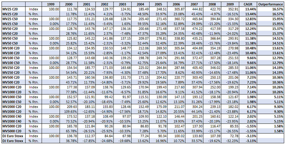
The results are hypothetical results and are NOT an indicator of future results and do NOT represent returns that any investor actually attained. Indexes are unmanaged, do not reflect management or trading fees, and one cannot invest directly in an index.
The NCAV MV25 C20 generated a CAGR of 13.44% vs the DJ Euro Stoxx -3.13%, an outperformance of 16.57%!
We chart below the CAGR of the 20 stock portfolios (i.e. “C20”) along with that of the market:
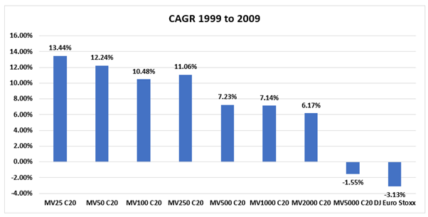
The results are hypothetical results and are NOT an indicator of future results and do NOT represent returns that any investor actually attained. Indexes are unmanaged, do not reflect management or trading fees, and one cannot invest directly in an index.
While, it appears as though the “cheapest” firms produced market-beating return from 1999 to 2009 in the Eurozone across a full spectrum of market capitalizations, when we examined returns by decile, the efficacy of the NCAV/MV metric was brought into question.
Below we restate the returns reported in the paper of decile 1 (D1) and decile 2 (D2) (minimum market capitalization 100m) alongside those of the MV100 C20 portfolio for comparative purposes:(21)
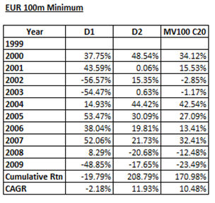
The results are hypothetical results and are NOT an indicator of future results and do NOT represent returns that any investor actually attained. Indexes are unmanaged, do not reflect management or trading fees, and one cannot invest directly in an index.
The MV100 C20 portfolio consists of the 20 firms that possessed the highest ratio of NCAV/MV i.e. the cheapest stocks. Therefore those 20 firms would be subsumed within D1. While the cheapest 20 firms generated a CAGR of 10.48% the cheapest decile, which contained those firms, generated a CAGR of -2.18%. Yet D2, which contained more expensive firms, generated a higher CAGR of 11.93%!
The above implies a lack of robustness to the hypothesis that cheapness, as measured by the NCAV/MV was the driver of returns, for if it was, we would expect a consistent reduction in returns as the NCAV/MV decreased (i.e. firms became more expensive), as opposed to the inconsistent sequence identified above.
Furthermore, it should be noted that the 10.48% CAGR achieved by the MV100 C20 portfolio excluded dividends, whereas the -2.18 CAGR of D1 included dividends, further confounding the results.
Conclusion on “Studying Different Systematic Value Investing Strategies on the Eurozone Market”
Initially, the CAGR achieved by portfolios across a wide spectrum of market capitalizations seemed to definitively indicate the firms with the highest NCAV/MV (i.e. the cheapest) reliably and consistently outperformed the market as measured by the DJ Euro Stoxx. However, the robustness of the results was brought into question when we analysed the returns to the decile portfolios which revealed an inconsistency which could not be explained.
Detailed analysis: Analyzing Deep Value in the Eurozone.
What Has Worked in Investing (Tweedy Browne)
Celebrated value investors Tweedy, Browne Company LLC published a booklet in 2009 that contained over 50 studies titled “What Has Worked in Investing: Studies of Investment Approaches and Characteristics Associated with Exceptional Returns”. Contained therein was a study whose objective it was to examine the performance of securities that were selling at 66% or less of their NCAV from April 1970 to April 1981, thereby creating a 12 year study period.
Results and Analysis
The study included firms with market capitalizations as low as “$1 million”, which, even by today’s inflation-adjusted standards is likely to have resulted in the manifestation of uninvestable stock bias.
Table 4 from What Has Worked in Investing is reproduced below:
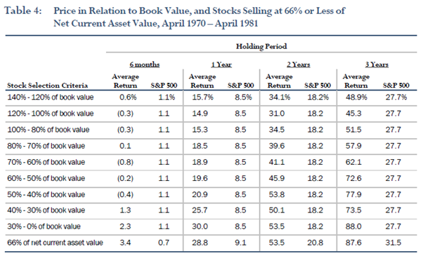
The results are hypothetical results and are NOT an indicator of future results and do NOT represent returns that any investor actually attained. Indexes are unmanaged, do not reflect management or trading fees, and one cannot invest directly in an index.
The “Average Return” is almost certainly the arithmetic mean occasioning in inflated return bias. We reached this conclusion as a number of other studies published in the booklet expressly state that returns were “compounded”, whereas in this case no such specification was made. Furthermore, using historical data we found that the specified 1 Year S&P500 of 8.5% reconciles almost perfectly to the S&P500 arithmetic mean return calculated using calendar year returns.(22) Oddly, the 1 Year S&P500 return presented against “Stock Selection Criteria” “66% of net current asset value” is different to all other portfolios (i.e. 9.1% vs 8.5%). Presumably, this is because a different time period was used for these portfolios, but we did not note any explanation for this difference in the study.
Conclusion on “What Has Worked in Investing” (Tweedy Browne)
In addition to time period bias (12 years) the study is almost certain to have also suffered from inflated returns bias and is highly likely to have been afflicted by uninvestable stock bias also.
While we did not expect well renowned practitioners to produce practically inapplicable research our analysis nonetheless provides a reminder as to why one should actively go in search of disconfirming evidence and question everything, irrespective of its source.
“The important thing is not to stop questioning.”
Albert Einstein
Detailed analysis: What Has Worked in Investing (Tweedy, Browne) – Examining Net Nets
Emerging Markets: Evaluating Graham’s Stock Selection Criteria on Portfolio Return in Saudi Arabia Stock Market
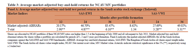
“Emerging Markets: Evaluating Graham’s Stock Selection Criteria on Portfolio Return in Saudi Arabia Stock Market” by Nadisah Zakaria and Fariza Hashim examined the performance of securities that were trading at greater than 1.5 of their Net Current Asset Value (NCAV)/Market Value (MV) (i.e. less than 2/3 of NCAV) during the 15 year period from 2000 to 2014 on Tadawul (i.e. the Saudi Arabian Stock Exchange). The Tadawul possessed a market “capitalization of USD385.3 million” as “of 31st December 2011”.
Results and Analysis
The study encompassed a small sample size (fewer than 10 firms were eligible for investment in the years from 2007 to 2011 inclusive) and no minimum market capitalization requirement was imposed.
Table 3 summarizing the relevant returns is reproduced below:
The results are hypothetical results and are NOT an indicator of future results and do NOT represent returns that any investor actually attained. Indexes are unmanaged, do not reflect management or trading fees, and one cannot invest directly in an index.
What are “buy-and-hold abnormal returns (BHAR)”? In essence, in this instance, the BHAR represents the geometric mean return less the market return.
So, while equally weighting (“EWI”) and holding 12 months produced a 20.17% BHAR the next question that comes to mind is, “what was the equally weighted market return that was outperformed by 20.17%”? Unfortunately, this was not reported.
In addition, it is worth noting that value weighting (“VWI”) resulted in a materially lower BHAR implying that the smaller companies were driving the “abnormal returns”.
Conclusion on “Emerging Markets: Evaluating Graham’s Stock Selection Criteria on Portfolio Return in Saudi Arabia Stock Market”
The study suffered from time period bias (15 years) and the sample size examined was particularly small. Significantly, the study is also highly likely to have suffered from uninvestable stock bias given that no minimum market capitalization requirement was imposed. Furthermore, the market addressed possessed a capitalization of less than USD 400m raising further concerns with regard to liquidity. Also noteworthy is that regulatory restrictions during the study period would have prevented foreign investors from being able to access the potential opportunities.
Detailed analysis: Examining Saudi Arabian Net Nets
An Empirical Analysis of Ben Graham’s Net Current Asset Value Rule
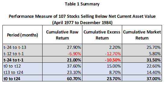
“An Empirical Analysis Of Ben Graham’s Net Current Asset Value Rule” by Joseph D Vu was published in The Financial Review (1988) and it examined the performance of securities that were trading at less than their NCAV during the 8 year period from 1977 to 1984 on the New York Stock Exchange (NYSE) and American Stock Exchange (AMEX).
Results and Analysis
The study suffered from a small sample size post-1977 and presented, in all likelihood, arithmetic mean returns (i.e. “Raw Returns”) resulting in inflated return bias. In addition, no minimum market capitalization was required for the securities under examination.
From Table 1 in the study we calculate and summarise the monthly return statistics from both before (t-24 to t-1) and after (t0 to t24) a security traded below its NCAV, and therefore qualified for investment. For reference we also quantify and report the cumulative market return (which was not reported in the original study):
The results are hypothetical results and are NOT an indicator of future results and do NOT represent returns that any investor actually attained. Indexes are unmanaged, do not reflect management or trading fees, and one cannot invest directly in an index.
Observing the cumulative excess return graphically reveals much:
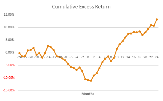
The results are hypothetical results and are NOT an indicator of future results and do NOT represent returns that any investor actually attained. Indexes are unmanaged, do not reflect management or trading fees, and one cannot invest directly in an index.
Post-event returns turn positive almost immediately. In the first year, the cumulative raw return was 37.60% versus 22.60% for the market, an excess return of 15.00% (i.e. a 66.37% outperformance). For the total two year post-event period the cumulative raw return was 60.70% versus 37.00% for the market, an excess return of 23.70% (i.e. a 64.05% outperformance).
From the breakdown of the return statistics, it appears that the first year post-formation resulted in the bulk of return suggesting that a one-year rebalancing period may prove to be return enhancing.
From April 1977 to December 1984 it appears as though firms trading below NCAV on the NYSE and AMEX demonstrated near-perfect market timing capability – seemingly a magical time to be a deep value investor!
Conclusion on “An Empirical Analysis of Ben Graham’s Net Current Asset Value Rule”
In addition to time period bias resulting from the 8 year examination period, the study is also likely to have suffered from inflated return bias and was exposed to uninvestable stock bias.
Detailed analysis: Examining “An Empirical Analysis of Ben Graham’s Net Current Asset Value Rule”
How the small investor can beat the market
“How the small investor can beat the market” by Joel M. Greenblatt, Richard Pzena and Bruce L. Newberg was published in the Journal of Portfolio Management (1981).(23) The paper was their Master’s thesis while studying at Wharton business school. The objective of the paper was to largely examine the performance of positive earning securities that were trading at or below their “liquidation value” during the 6 year period from April 1972 to April 1978 in the US.
Results and Analysis
While a minimum market capitalization of “over $3 million” was required for a stock to be considered, even after adjusting for inflation stocks close to the stipulated $3 million cut off may still have been insufficiently liquid to enable trading to occur in a “reasonable manner”. In addition, one needs to bear in mind that the researchers had to manually collect the necessary data thereby increasing the risk of human error.
Table 1 summarizing the portfolio returns has been reproduced below:
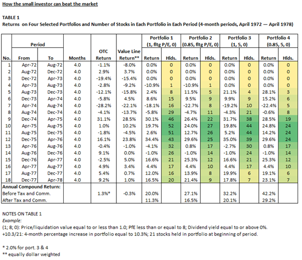
The results are hypothetical results and are NOT an indicator of future results and do NOT represent returns that any investor actually attained. Indexes are unmanaged, do not reflect management or trading fees, and one cannot invest directly in an index.
If you immediately and intuitively understand the data in Table 1 we refer you to the following:
“I know you think you understand what you thought I said, but I’m not sure you realize that what you heard is not what I meant”
attributed to Alan Greenspan
A few points (which are covered in greater depth in our detailed analysis) are warranted:
- “Period” returns do not reconcile to the “Annual Compound Return” specified at the foot of the table.
- Annual Compound Returns – we assume the Annual Compound Returns were calculated by applying the stated sell strategy/holding period whereby the authors “sold a stock after a 100% gain or after 2 years, whichever came first”.
- Sample Size – the average portfolio contained 15 stocks and ranged from 0 to 52.
- Dividends – the Annual Compound returns did not include dividends and are therefore understated (during the test period “Dividends averaged between 3% and 4% annually”).
- Taxes, Commissions and slippage – “we assumed commissions of 2.5% on purchase price plus a 2.5% bid/ask spread (the bid/ask spread was applied to the 60% of our stocks that were purchased over-the-counter), a 2.5% commission on selling price, and a 25% capital gains tax (over 90% of the stocks were held long enough to qualify for capital gains treatment).” The commissions included are in line with the higher trading costs associated with the time period examined.(24)
- P/E floating with bond yields – “We required a P/E corresponding to twice the prevailing triple A yield in each period (e.g. triple A yield = 8%; required PPE equal or below the reciprocal of 16%, or 6.25).” The Triple A bond yield during the period studied ranged from approximately 7 to 9 implying a requirement for a P/E below 5.5 to 7.(25) This means that the P/E requirement of ≤ 5 for Portfolio 3 and 4 was less than the maximum floating P/E allowed for Portfolio 1 and 2.
Having laid out the above we are better placed to analyse the results, bearing in mind the relatively small sample size, notwithstanding that the authors “attempted to select a statistically significant and unbiased sample of stocks”.
The highest returning portfolio was Portfolio 4 (42.2%) which required stocks in the portfolio to possess the lowest valuation in terms of both liquidation value (≤ 0.85) and P/E ratio (≤ 5.0).
Interestingly, Portfolio 3 (32.2%) returned more than Portfolio 2 (27.1%) despite its allowance for a higher liquidation cut off (≤ 1.0 vs. ≤ 0.85 for Portfolio 2) but a lower P/E threshold (≤ 5.0 vs ≤ ~5.5 to 7 for Portfolio 2).
Portfolio 1 which allowed for the highest valuation in terms of liquidation value (≤ 1.0) and P/E (≤ ~5.5 to 7) generated the “lowest” return (20.0%).
Overall, the results imply valuation drives futures returns, however, the merit of liquidation value vs the P/E ratio to explain future returns is less clear.
In terms of relative returns all portfolios greatly outperformed the “OTC” and “Value Line” portfolios which generated an Annual Compound Return (before taxes and commissions) of 1.3% and -0.3% respectively. Significantly, the outperformance of all portfolios survived taxes, commissions and slippage. However, all returns during the period were severely impacted by the ravages of inflation which averaged approximately 7.5% per annum (geometric mean) from 1972 to 1976.(26)
Conclusion on “How the small investor can beat the market”
“How the small investor can beat the market” demonstrated that the Annual Compound Returns for firms with positive earnings trading at or below liquidation value, combined with a low price to earnings ratio greatly outperformed OTC and Value Line firms during the examination period (April 1972 to April 1978), even after taking into account taxes, commissions and slippage.
That said, the examination period (6 years) was simply too short to provide definitive guidance as to the efficacy of investing in firms trading at or below liquidation value. Furthermore, the study may have suffered from uninvestable stocks bias and it also harbored a number of idiosyncrasies which we highlighted in our detailed analysis. In aggregate, the study represents a small, though not untainted piece in the larger puzzle of determining what we “really know” about returns of such firms from an empirical standpoint.
Detailed analysis: Examining Greenblatt’s “How the small investor can beat the market”
Testing Benjamin Graham’s net current asset value model
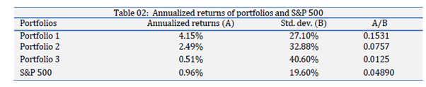
“Testing Benjamin Graham’s net current asset value model” by Chongsoo An, John J. Cheh , and Il-woon Kim published in Journal of Economic & Financial Studies (2015) examined the performance of securities that were trading at less than their NCAV during the 14 year period from January 2, 1999 to August 31, 2012 in the US market.
Results and Analysis
The authors presented “annualized returns” (i.e. CAGR). “The annualized returns of three portfolios and S&P 500 during the study period are presented in Exhibit 2. Annualized returns are the returns that should have been realized every year to earn total returns during the study period. Theoretically, the stocks with a higher NCAV/MV value should be generating annualized returns higher than the stocks with a low value. The results of this study, however, are mixed. Portfolio 1 (4.15%) and Portfolio 2 (2.49%) beat the market with a big margin as shown in Exhibit 2, while Portfolio 3 (0.51%) does not do well compared to the S&P500 (0.96). It is also puzzling to see in Exhibit 2 that the returns are decreasing as the value of N is increasing from 1 to 2 and to 5. We believe that these mixed results are due to the fact that the number of firms in each portfolio is decreasing from 84, to 31 and to 10. As the sample size is getting smaller, the results of the study are getting less reliable and sometimes inconsistent.”
It should be noted that the sample size was particularly small as disclosed in the narrative. In addition, no minimum market capitalization was specified for the securities examined thereby exposing the results to the perils of uninvestable stock bias.
Interestingly, the Portfolio returns were in the opposite sequence to that which was expected. “It was expected that the stocks with a higher NCAV/MV value (e.g., N=5) would be generating returns higher than the stocks with a low value (e.g., N=1).”
What is particularly interesting about these results is the low level of absolute return outperformance relative to the market when compared to the other studies examining the returns to firms trading below NCAV. For example, for Portfolio 1, the best performing portfolio, the absolute outperformance relative to the S&P 500 was just 3.19% (4.15%-0.96%). Furthermore, net of fees and commissions the absolute return outperformance would have been even lower. Indeed, the annualized return to three-month Treasury bills over the 14 year period was approximately 2.3%; a figure reasonably comparable to the net of fee and commission return likely to have been achieved.
(27) Furthermore, net of taxes (and effort) investing in firms with an NCAV > MV (i.e. trading at a discount to NCAV) appears to have been a forlorn endeavor in the US market over the test period.
The “average” (i.e. arithmetic mean) returns were reported as follows:
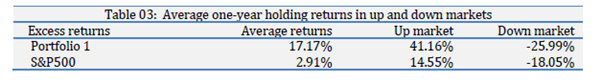
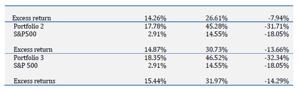
Recall the annualized returns (CAGR/geometric mean) for Portfolio 1, 2 3 and the S&P 500 was 4.15%, 2.49%, 0.51% and 0.96% respectively. In contrast the “simple averages [i.e. arithmetic mean] of all rebalancing returns realized in backtesting… with one year holding period” for Portfolio 1, 2, 3 and the S&P 500 was 17.17%, 17.78%, 14.87% and 2.91% respectively.
Using Portfolio 1 as an example, that represents a 13.02% return differential (17.17% – 4.15%). To illustrate the magnitude of that differential, compounding $100,000 at the Portfolio 1 annualized return rate of 4.15% yields $176,696 (100,000*(1.0415)^14-1) over 14 years (the length of the study period). In contrast, wrongly assuming that one could “compound” at the (arithmetic) average rate of 17.17% per Portfolio 1 would result in the mistaken belief that a terminal value of $784,537 (100,000*(1.1717)^14-1) was achievable. That represents a $607,841 (or 77.5%) difference in potential expectation.
The authors also examined a “Hedging Strategy” which reported impressive results, however, we believe it lacked robustness. We examined it in our detailed analysis along with the reported returns achieved by utilizing different holding periods.
Conclusion on “Testing Benjamin Graham’s net current asset value model”
Despite the quantification of annualized returns, the study cannot be considered reliable due to its likely exposure to uninvestable stock bias. In addition, the particularly small sample size of securities meeting the necessary criteria is also of concern.
Conveniently, the authors also presented the arithmetic average returns which provided a timely, relevant and objective lesson into why attempting to estimate the geometric mean from the arithmetic mean is an inadvisable action.
Reliability concerns notwithstanding, the study demonstrated that even over a 14 year period investing in firms trading below NCAV may not provide immunity from a low return environment – a sobering realization.
Detailed analysis: An Analysis of “Testing Benjamin Graham’s net current asset value model”
Ben Graham’s Net Nets: Seventy-Five Years Old and Outperforming
“Ben Graham’s Net Nets: Seventy-Five Years Old and Outperforming” by Tobias Carlisle, Sunil Mohanty, and Jeffrey Oxman (2010) aimed to provide an update on the research published by Henry R. Oppenheimer in his 1986 paper, “Ben Graham’s Net Current Asset Values: A Performance Update”.(28) Following the methodology adopted in Oppenheimer’s research, the authors selected securities that were trading at no more than two-thirds of their NCAV. Their 25 year examination period ran from 31 December 1983 to 31 December 2008 and they focussed on US-listed securities.
Results and Analysis
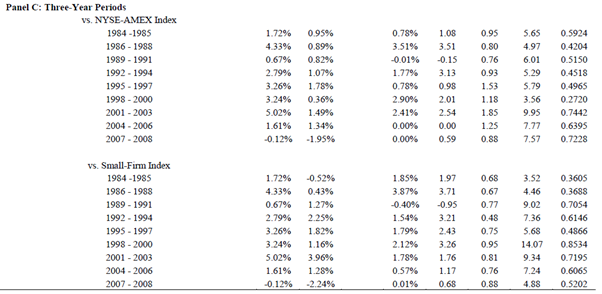
While this study purported to be an update of Oppenheimer’s 1986 study unfortunately it did not contain the all corresponding tables. Specifically, the most useful table from Oppenheimer’s study was Table IV which displayed the return in each year of the study and presented the “Annual Geometric Mean Return”.
12 Month Holding Period
“Exhibit 2 summarizes the results for the 25-year period of the study”, which deals with the 12 month holding period:
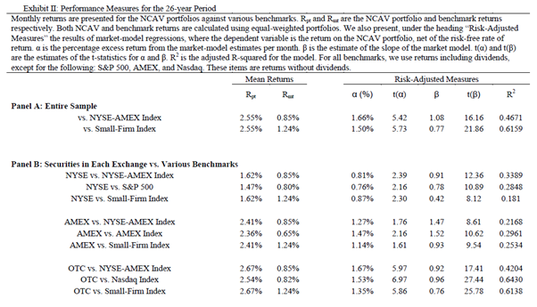
The results are hypothetical results and are NOT an indicator of future results and do NOT represent returns that any investor actually attained. Indexes are unmanaged, do not reflect management or trading fees, and one cannot invest directly in an index.
We note that the table heading states it is a “26” year period, however, the study covers 25 years.
They present “monthly” “Mean Returns” (i.e. arithmetic mean). Exhibit II does indeed replicate the data presented in Table II of Oppenheimer’s study. Furthermore, based on reconciliation work carried out in “An Analysis of Benjamin Graham’s Net Current Asset Values: A Performance Update”, it reinforces our view that the arithmetic mean returns have also been presented in this case. Therefore, the results have been afflicted by inflated return bias.
30 Month Holding Period
30 month holding periods are examined and presented in Exhibit III (partially reproduced below).
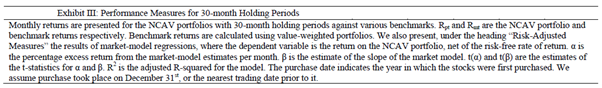
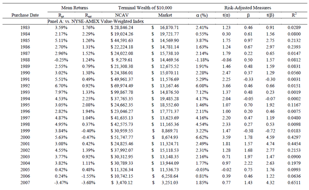
The results are hypothetical results and are NOT an indicator of future results and do NOT represent returns that any investor actually attained. Indexes are unmanaged, do not reflect management or trading fees, and one cannot invest directly in an index.
At first glance Exhibit III, through its measurement of the “Terminal Wealth of $10,000” appears to be the representation of the actual dollar return achievable by an investor in practice (i.e. geometric mean/compounded return). However, like we discovered in “An Analysis of Testing Benjamin Graham’s Net Current Asset Value Strategy in London” and “What Has Worked in Investing (Tweedy, Browne) – Examining Net Nets” researchers “compounded” the arithmetic mean in attempt to put the returns in more “meaningful terms”. Indeed, we believe this to be the case in this study also. For instance, the 1983 monthly mean return of 3.59% when compounded for the stipulated 30 months with a starting value of $10,000 yields (rounding aside) the reported ~$28,846.24 (10,000*(1.0359)^30). When 3.59% is compounded monthly it results an annualized (i.e. compounded) return of 55.7% ((28,846.24/10,000)^(12/30)-1). Similarly, in 1993 the reported monthly mean return was 7.97%. When $10,000 is compounded for 30 months at 7.97% it yields (rounding aside) the reported ~$99,867.78 (10,000*(1.0797)^30). When 7.97% is compounded monthly it results in an annualized (i.e. compounded) return of 151.1% ((99,867.78/10,000)^(12/30)-1).
The implied returns are as extraordinary as they are illusionary!
Earnings and Dividends
Exhibit 4 is reproduced below:
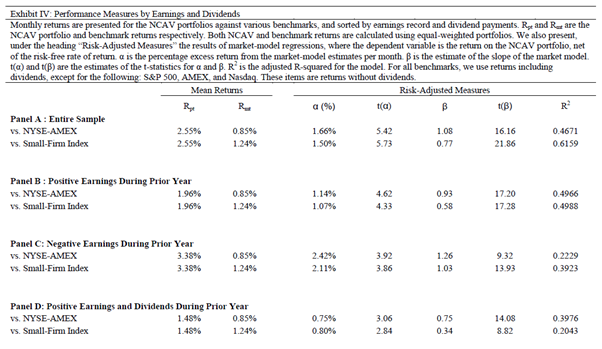
The results are hypothetical results and are NOT an indicator of future results and do NOT represent returns that any investor actually attained. Indexes are unmanaged, do not reflect management or trading fees, and one cannot invest directly in an index.
Having established that Oppenheimer’s results were compromised due to the exclusion of dividends we proceed by examining the same issue in this study.
The authors state, “Monthly returns are presented for the NCAV portfolios against various benchmarks and sorted by earnings record and dividend payments. Rpt and Rmt are the NCAV portfolio and benchmark returns respectively….For all benchmarks, we use returns including dividends, except for the following: S&P 500, AMEX, and Nasdaq. These items are returns without dividends.” Why total returns (i.e. including dividends) were not used with regard to the S&P 500, AMEX, and Nasdaq is unknown. While portfolios may have been sorted by “earnings and dividend payments”, it remains unclear whether the data used to measure the returns incorporated the dividend payments themselves.
“The results in this section indicate a rational connection between risk and return. Dividend-paying firms are viewed as less risky because the dividend signals to shareholders that managers believe the future cash flows of the firm are stable enough to accommodate an ongoing dividend.”
To accept the above conclusion an investor must also accept that “risk” is represented by the various “Risk-Adjusted” measures presented, along with their implicit association with price volatility. Indeed, the acceptance of “beta” as an appropriate measure of risk-adjusted returns runs contrary to the “low-beta anomaly”.(29)
Also, of concern is that no hypothesis (i.e. preceding the testing) was provided (in either study) for such results. Absent a more sound economic rationale for why positive earning non-dividend-paying firms, 2.42% (and negative earning firms, 3.38%) would generate higher returns than positive earning dividend-paying firms, 1.48% (and positive earning firms, 1.96%), data mining or the exclusion of dividends from the return data may provide greater explanatory power for the reported results compared to that provided within the study itself.
Valuation and Returns
Exhibit 5 and the corresponding narrative is reproduced below:
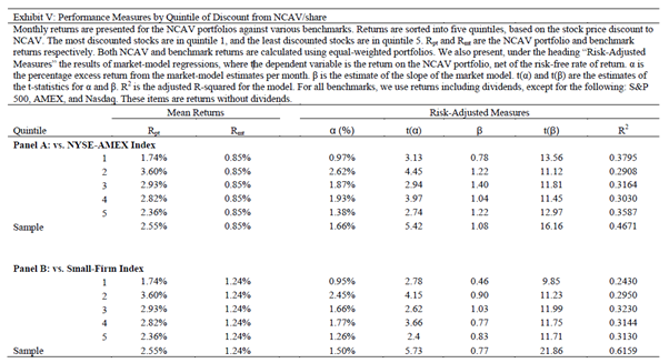
“Quintile 1 contains the fifth of the firms that have the highest discount, and Quintile 5 contains the firms trading closest to two-thirds of NCAV. With one caveat… the returns are higher for firms with higher discounts to NCAV. The caveat is as significant as it is perplexing: securities in Quintile 1– those with the lowest purchase price to NCAV – have the lowest returns. As noted earlier, we have eliminated as outliers firms with stock prices less than one percent of the NCAV per share, so we do not believe outliers are driving this result.”
Some food for thought pertaining to the reported results: in general, value investing research shows returns that are consistent with the relative “cheapness” of the underlying portfolios examined.(30) Firms trading at less than 2/3 of NCAV would, almost certainly, consist of firms that in aggregate sit in the bottom decile of price to book (or by academic convention, the top decile of book to market). Perhaps then, sorting these firms again based on a discount to NCAV possess limited utility; rather, other metrics (e.g. “quality measures”) may be required to eliminate the relatively poor performers. Indeed, in “Analyzing Deep Value in the Eurozone” we also observed that the firms that traded in the cheapest decile sorted by relative price to NCAV produced lower returns than those in the second cheapest decile.
As such then, we have no definitive explanation regarding the above results and only proffer thoughts for further contemplation.
Explanations for Excess Returns
The authors attempted to explain the “excess returns” by regressing a number of factors against the NCAV returns. For interested readers we recommend reviewing the underlying paper, however, we nonetheless provide the key extract from the paper below:
“we are confident that the market risk, small-firm effect (SMB) and liquidity factors (ILLIQ) are the only [our emphasis] factors that explain the returns on the NCAV portfolios of the ones we have applied.”
Indeed, the results of the regression analysis may elicit a range of reactions. Some may consider the results to be “objective and instructive”, while for other the results may evoke the quote, “Lies, damned lies, and statistics”!
We leave it to readers to ascertain the utility, or otherwise, of that presented by the authors in this section.(31)
Minimum market capitalization requirement
No minimum market capitalization requirement was specified for the securities examined and therefore the results are highly likely to have suffered from uninvestable stock bias.
Conclusion on “Ben Graham’s Net Nets: Seventy-Five Years Old and Outperforming”
The authors conclude, “The results are as clear as they are compelling: Seventy-five years on, Graham’s NCAV rule continues to identify securities that generate above-market returns.”
When looking at the findings reported in the paper from a practitioner’s point of view, our conclusion is different. The study suffered from inflated return bias and is also highly likely to have been impacted by uninvestable stock bias. For the practitioner not afraid to be confronted with a conclusion that may be inconsistent with their prior beliefs, we offer our version of the authors conclusion based on our extensive analysis of the study:
“The results are as clear [unclear] as they are compelling [overstated]: Seventy-five years on, Graham’s NCAV rule continues to identify securities that [may] generate above-market returns, [we simply do not know based on the methodology adopted in this study].”
Detailed analysis: Examining “Ben Graham’s Net Nets: Seventy-Five Years Old and Outperforming”
The Verdict
Graham’s genius and intestinal fortitude in developing the strategy of investing in firms trading below their NCAV was remarkable, especially when one considers the era in which it transpired. Despite that, the research examining the strategy has been relatively limited when compared to the volume of investment literature published on more commonly discussed valuation metrics. Due to the remarkable returns reported in many of the studies our objective was to determine if “the returns reported in the research could have been achieved by an investor in practice”. To answer this question and fulfil our objective we developed an extensive methodology to “analyse the evidence”.
When viewed from the perspective of a practitioner (as opposed to an academic researcher) our analysis revealed that the underlying research contained methodological shortcomings, often resulting in the inability for the reported returns to be attained in reality.
Specifically, of the ten studies examined five suffered from inflated return bias (among other issues) and we therefore disregard their results. Of the remaining five studies one did not actually examine the return to stocks trading below NCAV and we therefore disregard it also. Of the four remaining studies three were highly likely to have suffered from uninvestable stock bias, in addition to other issues previously detailed.
That leaves just one, study, “How the small investor can beat the market”, which was not beyond reproach either. The study examined a relatively small sample of firms during the six-year period from 1972 to 1978 in the US. Among other concerns, clearly, a study spanning just six years and examining just one market is insufficient to determine the efficacy of any investing strategy for it demonstrates both a lack of “persistence” and “pervasiveness”.(32)
In essence, then, an investor could have potentially, though not assuredly, achieved the returns reported in just one out of the ten studies examined.
We therefore conclude that when viewed from the perspective of a practitioner, the empirical evidence analysed is insufficient to support the view that investing in securities trading below their NCAV provides a reliable source of material outperformance.
Stated simply, “Could the returns reported in the research have been achieved by an investor in practice?” Essentially, no.
The Implications
Does our research suggest investing in firms trading below NCAV is a “bad strategy”? No, the “absence of evidence is not the evidence of absence”. By this, we mean the lack of robustness in, and insufficiency of, the empirical evidence pertaining to firms trading below NCAV does not prove that the strategy cannot generate market-beating performance.
Indeed, great investors such as Buffett, Schloss, Cundill and, of course, Graham himself advocated for the purchase of securities trading below a conservative liquidation value.(33) However, our analysis of the sample of research identified demonstrates that the performance capability of such a strategy remains largely unknown from a practitioner’s standpoint.
While our analysis focussed on the evidence concerning firms trading below NCAV and found it wanting, its implications resonate much further. For “evidence-based investors” it ought to evoke the questions, “How well do I understand the evidence on which I base my capital allocation decisions?”, “Can the returns reported in that evidence actually be translated into investment reality?”.
Being an evidenced-based investor sounds intelligent, understanding the evidence is being an intelligent investor.
We commenced with a quote attributed to Mark Twain and it seems only fitting that we conclude with another quote also attributed to him:
“It ain’t what you know that gets you in trouble, it’s what you know for sure that just ain’t so.”
References[+]
| ↑1 | Benjamin Graham and David Dodd. Security Analysis: Sixth Edition. McGraw Hill 2009, pg. 586; Graham also wrote about this strategy for Forbes in 1932, “Ben Graham Then and Now” (https://www.forbes.com/forbes/2008/1110/056.html#3f4004de21e4) |
|---|---|
| ↑2 | Benjamin Graham and David Dodd. Security Analysis: Sixth Edition. McGraw Hill 2009, pg. 553 |
| ↑3 | Tobias E. Carlisle. Deep Value, Wiley 2014, pg. 21 |
| ↑4 | Wall Street Crash of 1929, https://en.wikipedia.org/wiki/Wall_Street_Crash_of_1929 |
| ↑5 | More details here. |
| ↑6 | Kewei Hou, Chen Xue, Chen Xue, Lu Zhang , “Replicating Anomalies” (2017). https://papers.ssrn.com/sol3/papers.cfm?abstract_id=2961979. |
| ↑7 | Microcap Stock: A Guide for Investors: The term “microcap stock” applies to companies with low or “micro” capitalizations, meaning the total value of the company’s stock. A typical definition would be companies with a market capitalization of less than $250 or $300 million. The smallest public companies, with market capitalization of less than $50 million, are sometimes referred to as ‘nanocap stocks.’ (https://www.sec.gov/reportspubs/investor-publications/investorpubsmicrocapstockhtm.html) |
| ↑8 | Chee Seng Cheong A Fin, Justin Steinert, “The size effect: Australian evidence”, JASSA Issue 2 Winter 2007. |
| ↑9 | Approximately equal to an inflation-adjusted USD 31m in 2020. https://www.usinflationcalculator.com/ |
| ↑10 | Inequality of arithmetic and geometric means https://en.wikipedia.org/wiki/Inequality_of_arithmetic_and_geometric_means |
| ↑11 | Elton, E. and Martin Gruber, 1977, Risk Reduction and Portfolio Size: An Analytical Solution, The Journal of Business 50, p 415-437. |
| ↑12 | One could make an argument that the arithmetic mean return combined with the standard deviation may be “sufficiently” informative. However, when dealing with extreme return events assumptions pertaining to the nature of the underlying distribution of returns (i.e. normal distribution vs e.g. “Chebyshev Bound” ) and the corresponding confidence bound make the task unnecessarily complex and fraught with the need to make unnecessary assumptions. In contrast, the compound annual growth rate would provide the necessary information simply, accurately, and succinctly. |
| ↑13 | Wesley Gray and Jack Vogel, “Analyzing Valuation Measures: A Performance Horse-Race over the Past 40 Years.” https://papers.ssrn.com/sol3/Papers.cfm?abstract_id=1970693 |
| ↑14 | Wesley R. Gray, Jack Vogel, “Using Maximum Drawdowns to Capture Tail Risk”, 2013. https://papers.ssrn.com/sol3/Papers.cfm?abstract_id=2226689 |
| ↑15 | Anchoring (cognitive bias) https://en.wikipedia.org/wiki/Anchoring_(cognitive_bias) |
| ↑16 | A Century Of Stock Market Liquidity And Trading Costs, Charles M. Jones, Graduate School of Business Columbia University, 2002 (https://papers.ssrn.com/sol3/papers.cfm?abstract_id=313681);
We assumed our investor was in the highest tax bracket
|
| ↑17 | That said, also as a result of using data that excluded dividends, it is theoretically possible that the reported returns may have been generally understated throughout the study depending on the impact, if any, of including firms that may have been untradeable. |
| ↑18 | http://www.stern.nyu.edu/~adamodar/pc/datasets/histretSP.xls |
| ↑19 | We were able to get in contact with the author, Glen Arnold, Ph.D. and he confirmed that “Each post-portfolio formation month has a number, 1, 2, 3 etc. The returns are measured for the post-portfolio month e.g. month 35, for each of the portfolios starting in different years. They are then simply averaged arithmetically.” |
| ↑20 | Confirmed by an author. |
| ↑21 | D1 contains the firms highest NCAV/MV ratio i.e. the cheapest. |
| ↑22 | http://www.stern.nyu.edu/~adamodar/pc/datasets/histretSP.xls |
| ↑23 | MarketFox Interview with Rich Pzena in which he briefly discusses the study (https://i3-invest.com/podcasts/i3-podcast-marketfox-interview-with-rich-pzena/) |
| ↑24 | A Century Of Stock Market Liquidity And Trading Costs, Charles M. Jones, Graduate School of Business Columbia University, 2002 (https://papers.ssrn.com/sol3/papers.cfm?abstract_id=313681) |
| ↑25 | https://fred.stlouisfed.org/series/AAA |
| ↑26 | https://www.inflation.eu/inflation-rates/united-states/historic-inflation/cpi-inflation-united-states.aspx |
| ↑27 | http://pages.stern.nyu.edu/~adamodar/New_Home_Page/datafile/histretSP.html |
| ↑28 | We contacted the corresponding author on a number of occasions to seek clarity on aspects of the study and never received a response, nor did we receive a response from the second listed author, and the first listed author did not have in his possession the underlying data which we wished to review. |
| ↑29 | For research on Low-Volatility/Low-Beta see here: https://alphaarchitect.com/category/architect-academic-insights/factor-investing/low-volatility-investing/ |
| ↑30 | For further value investing research see here: https://alphaarchitect.com/category/architect-academic-insights/factor-investing/value-investing/ |
| ↑31 | The same research team (Tobias Carlisle, Sunil Mohanty, and Jeffrey Oxman) authored the paper “Dissecting the Returns on Deep Value Investing” (2012) (https://papers.ssrn.com/sol3/papers.cfm?abstract_id=1928694 ) in which they examined numerous factors in an attempt to “explain the returns” to firms trading below NCAV (albeit with a variation of the valuation methodology applied in this study). |
| ↑32 | Andrew L. Berkin , Larry E. Swedroe, “Your Complete Guide to Factor-Based Investing: The Way Smart Money Invests” (2016). “Persistent – It holds across long periods of time and different economic regimes”, “Pervasive – It holds across countries, regions, sectors, and even asset classes”. |
| ↑33 | Though none, to our knowledge, advocated for the indiscriminate buying of securities purely on the basis of their trading below NCAV. |
About the Author: Gaurang Merani, CPA
—
Important Disclosures
For informational and educational purposes only and should not be construed as specific investment, accounting, legal, or tax advice. Certain information is deemed to be reliable, but its accuracy and completeness cannot be guaranteed. Third party information may become outdated or otherwise superseded without notice. Neither the Securities and Exchange Commission (SEC) nor any other federal or state agency has approved, determined the accuracy, or confirmed the adequacy of this article.
The views and opinions expressed herein are those of the author and do not necessarily reflect the views of Alpha Architect, its affiliates or its employees. Our full disclosures are available here. Definitions of common statistics used in our analysis are available here (towards the bottom).
Join thousands of other readers and subscribe to our blog.