Jack Bogle, the founder of Vanguard, created a simple explanation for predicting future stock returns. The so-called “Occam’s razor” (law of parsimony) approach is an attempt to explain projected returns as simple as possible.
Mr. Bogle’s model is pretty simple:
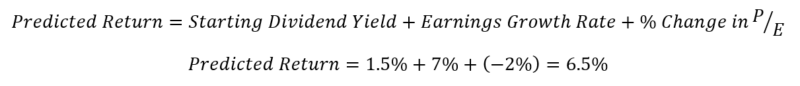
Expected returns (nominal, annualized over the next 10 years) = Starting Dividend Yield + Earnings Growth rate + Percentage change (annualized) in the P/E multiple.
Source paper link

Not bad! A simple three-factor model to predict stock returns.
The starting dividend yield is known. Earnings growth rates can be estimated using prior data. And changes in the P/E multiple can be approximated—but of note—this is the hardest variable to predict.(1)
How did this model do?
Let’s look at two examples in the past.
All information is on the S&P 500 index, with the (1) Dividend Yield, (2) EPS, and (3) P/E multiples from multpl.com, as this is a source that anyone can easily view data.(2)
As many investors remember, from 1/1/2000-12/31/2009, nominal returns to owning the S&P 500 of an annualized negative 0.95% over 10-years!(3)
With the benefit of hindsight, what would the model have predicted?
Below is an image using snapshot data as of ~ 1/1/2020 and 1/1/2010—a 10-year period.
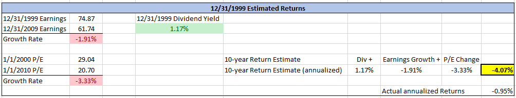
The model would have predicted an even worse return—negative 4.07% annualized return.
Why?
This was driven by (1) the aggregate S&P 500 earnings (Earnings-per-share—EPS) declining for a decade and (2) multiples compressing from a P/E multiple of 29 to a P/E multiple of 21.
What about a good equity return period?
Well, the next decade was a great time to be an equity investor—a simple buy and hold investor owning the S&P 500 would have earned 13.57% from 1/1/2000 through 12/31/2019.
So, once again, with the benefit of hindsight, what would the model have predicted?
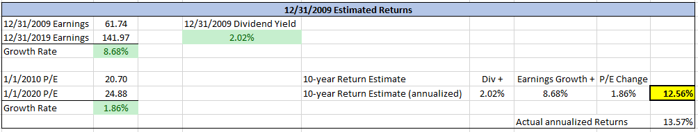
The model would have predicted a positive 12.56% annualized return.
This was driven by (1) P/E multiples expanding from 21 to 25 and (2) earnings growing at around 8.7% annualized for a decade!
Of course, we are using the inputs that we know, after the fact!
Thus, if we want to predict stock returns we need to come up with ways to estimate (1) the earnings growth rates and (2) the P/E multiple expansion/compression. Not exactly an easy task and it’s likely impossible to get the short-term (and even intermediate-term) predictions correct.
A PDF version of this article is available here.
Building a Model to Predict Stock Returns
Let’s walk through one example of how we can use Bogle’s model to predict stock returns—with the obvious caveat that this is only one model and is not guaranteed.
1. Starting dividend yield
This is the simplest part!
As of 3/10/2021, the dividend yield on the S&P 500 is ~ 1.50%.
2. Estimating the Earnings Growth Rates
The simplest way to estimate earnings growth rates is by using historical averages.
Here, one can either use geometric or arithmetic averages. One can also vary the look-back period.
Below are the numbers over numerous periods through 2019.(4)
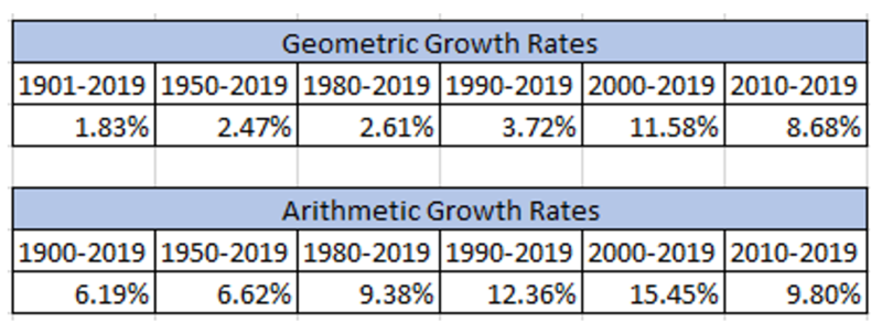
As we see, on average, over the long-run, firms grow their earnings. This makes sense as CEOs are incentivized in their compensation packages to maximize shareholder value.(5)
So, using the simple method of using averages, reasonable growth rates for earnings would be within the 4% – 12% range, using the past 30 years and examining both the average and geometric means.
Another approach, which is more complicated, involves a more detailed model to generate earnings growth rates. This involves projecting (1) future revenue growth for the market and (2) future profit margins. We examine these topics in detail in this post here (section 3 of the article).
The first item, future revenue growth, can be reasonably approximated by a combination of GDP and inflation (depending on the real/nominal GDP values). The second item needed is profit margins. Examining our old post, one of the biggest issues (looking back) was that our simulation assumed margins would mean-revert, on average. But margins actually increased! While difficult to say with certainty, there is a reasonable theory that profit margins may be permanently higher due to economic moats driven by technology—thus future margins may be higher than the long-term historical average. Thus, one can use a more complicated model to generate future earnings growth rates for the economy.
Here, we will stick with the simple model, and use 7% for the earnings Growth rate.(6)
3. Estimating the P/E multiple move
As Bogle and Nolan (2015) so nicely outline—over very, very long time periods—the majority of the returns to the stock market are generated by items (1) and (2)—dividend yield and earnings growth—which they call “Investment Return”. The last part, the change in P/E, they call “speculative return” as this is more prone to the whims of the market:
- If people are more risk-averse, multiples will be lower
- If people are less risk-averse, multiples will be higher
Of course, that is my oversimplification of the idea, and there are many other factors involved (inflation, interest rates, tax law, etc.).
In their paper, they highlight the prior returns to the market in Exhibit 1:
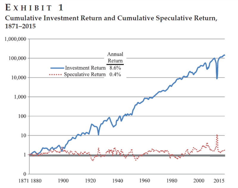
Over the long-run, dividends and earnings growth drive the returns, so by their model, these are the real important factors for predicting stock returns for very long time horizons.
However, not everyone has a 50-year+ time horizon, and 10-year periods can be prone to large changes in the P/E multiple!
Thus, we need to generate some model to figure out how multiples expand/contract over time.
Campbell and Shiller (1988 and 1998 papers) examined the idea of price-to-earnings (P/E) multiples being related to future stock returns. Their CAPE Ratio (Cyclically Adjusted Price to Earnings ratio) was used to examine future stock returns. The CAPE ratio is a nice method to normalize earnings and account for inflation.
In their papers (1988 and 1998), they found a high relationship between CAPE and future returns—higher CAPEs indicated lower returns in the future, and lower CAPEs indicated higher returns in the future.
In fact, their 1998 paper even highlighted that the P/E multiple, and specifically the CAPE multiple, was very high at the time (near the end of the Internet Bubble), and their model predicted that returns in the future will be low/negative.
And they were correct!
As shown above, the returns in the 2000s were negative for equity investors.
So why don’t we just use the CAPE model?
Well, I started with Bogle’s approach as I like the simplicity.
The other reason, as outlined in the 2019 JPM article, “Improving U.S. Stock Return Forecasts: A “Fair-Value” CAPE Approach” by Davis et al., is that the CAPE model has not worked too well out of sample.
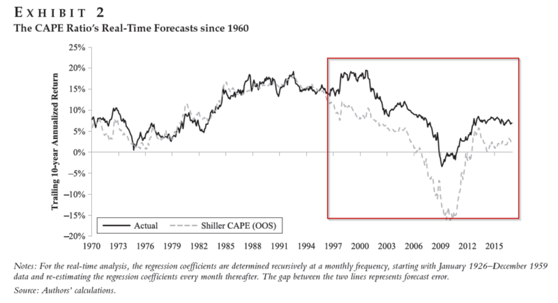
Exhibit 2 of the paper examines the performance of the CAPE model. As can be seen below, in my edited screenshot, the model worked very well for a long period of time.
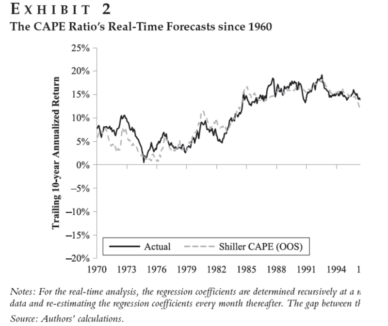
Unfortunately, out of sample, the CAPE model consistently predicted lower returns than what was realized in the market.
But why did this occur?
Well, the CAPE model requires a reversion to the mean. By this, I mean the model will predict that the current CAPE ratio will revert to the mean or the historical average.
Thus, if the CAPE is below the mean, the model will predict an expansion of the earnings multiple, which is “positive” to the predicted stock returns (it adds to the predicted returns). If, on the other hand, the CAPE is above the mean (which it currently is), the model will predict a contraction of the earnings multiple, which is “negative” to the predicted stock returns (it subtracts from the predicted returns).
Thus, this CAPE or P/E reversion effect can either increase or decrease predicted stock returns.(7)
But what if the mean has permanently changed? If so, the model would be “misspecified” as we’d assume reversion to the incorrect mean.
Davis et al. examine this question in their paper, as shown in Exhibit 3:
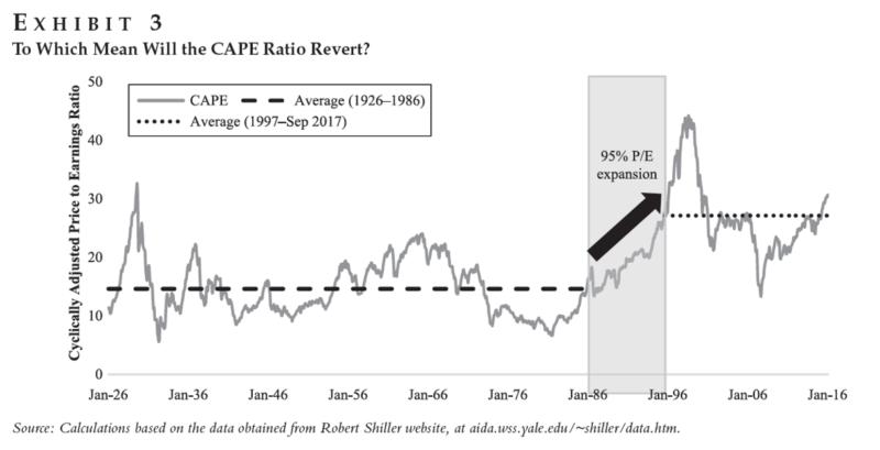
From this image, we see that there does appear to be a significant upward shift in the CAPE ratio over the past 30+ years, relative to the prior ~ 60+ years. Their solution is to edit the model to better predict the “mean reversion” or “the P/E change” part of Bogle’s formula. Details in this reference.(8)
Without diving too much into the model (and whether it is good/bad), the big idea is the following—these variables are predictive of the earnings yield, or the market multiple. In doing so, as opposed to only using the past CAPE ratio’s mean, they attempt to predict the future CAPE ratio—which in turn predicts the last part of Bogle’s formula—the change in the P/E multiple.
Not surprisingly, they find that this model works better than the simple CAPE model.
However, let us stick with the simple Bogle model for now (and even my simplification of the model), and try to predict the last variable we need—the change in the P/E multiple.
As of 3/10/2021, the S&P 500 is trading at ~3,900. Using the 2019 earnings value of ~ $142 as the baseline the current P/E multiple is 3900/142 ~ 27.5.
Important note–I am using the 2019 earnings as the 2021 earnings are generally expected to be near the 2019 earnings values. There are valid arguments for/against this approach as opposed to using the 2020 ending earnings of ~ $100. Obviously, if one believes that the covid impact is permanent and long-lasting, then you’d want to use the 2020 earnings number of $100. If, on the other hand, you believe that the impact is temporary, using the 2019 number as a baseline makes more sense.
Over the past 30 years, using annual data as of 12/31 each year, the S&P500 was trading at an average multiple of ~ 24 (the mean) and a median multiple of 21.
So, in our calculation—I am going to use a reversion to a P/E of 22.5 (average of the median and the mean).
Thus, the change in P/E, annualized over 10 years, is (22.5/27.5)^(1/10)-1 = -1.98%.
For simplicity, let’s say negative 2%.
Thus, if the P/E multiple contracts (as in my calculation) to a value of 22.5, the last part of Bogle’s equation would imply that changes in the P/E multiple will add a negative 2% annually to the market return annually over the next 10 years.
Putting it all Together to Predict Stock Returns
Thus, we have used one model, Jack Bogle’s model, and generated the three parts of the (nominal) predicted returns.
What one notices is that the predicted stock return is lower than in the past (many cite 10%+ annually).
Of course, this is only one model and is not guaranteed.
Below is a range of outcomes using the simple model by varying (1) the next decade’s growth rate of earnings and (2) the ending P/E of the market, with the assumption that (1) the starting dividend yield is 1.5% and the starting P/E is 27.5:
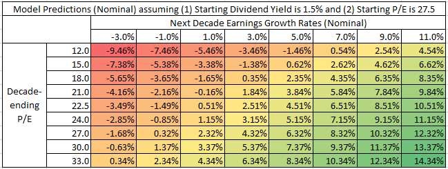
However, this is a simple model to use when attempting to figure out future returns. In the appendix below, I list links to other models/predictions.
Two items to note:
- Some models predict real returns and others predict nominal returns. Please be aware of the differences from firm to firm. In the model above, my prediction was nominal (before inflation).
- The largest variation in the predicted returns across the various models comes from “part 3” of the Bogle model—some firms expect a full reversion to the mean, while others may completely ignore this aspect
Hopefully, my prediction of 6.5% is way too conservative!
One note—this article highlights an image showing the long-term return is mainly driven by what Bogle calls the “Investment Return” while the “Speculative return” is close to 0. To see this, let’s be very bearish on long-term P/E multiples, and say that in 50 years, the P/E is going to 15.
Well—this means that from a starting P/E multiple of 27.5, its annualized impact on the total return (predicted) is (15/27.5)^(1/50)-1 = -1.2%. Thus—while this would have a negative impact, over the long-term, (1) dividends and (2) earnings growth should (hopefully!) subsume this number.
Appendix
- Campbell and Shiller’s paper – CAPE model in detail and how it was studied academically.
- Fight the Fed model – The main takeaway to remember: While the Fed Model can be good at describing how the market P/E is currently set, it is no better at predicting future stock returns than a model based on long-term P/E ratios.
- Vanguard expected returns (2021 version)
- AQR expected returns (2021 version) – Different models (in “real” terms, not nominal).
- Morningstar summary of 2021 expected returns
- Damodaran equity risk premium models – to get a predicted return, you add the equity risk premium (ERP) to the 10-yer T-bond yield at the time.
- Alpha Architect how to build expected return models.
- Research Affiliates expected returns module – note you can toggle between real and nominal returns, as well as change the “expected returns model”.
- A one-factor model by Cliff Asness to predict stock returns.
References[+]
| ↑1 | More on that below. |
|---|---|
| ↑2 | Of note, Shiller has data on his site as well, I just viewed this website as easier for anyone to “check” my calculations and view the data. |
| ↑3 | That is nominal returns, not real returns which account for inflation. |
| ↑4 | Using annual values, as opposed to monthly values. |
| ↑5 | In general the incentives are higher now than they were in the past, as the majority of the academic literature highlighting that CEOs with “pay packages aligned to shareholder value” started in the early 1990s—thus, more recent growth rates are probably applicable for the future if we assume incentives matter. |
| ↑6 | Giving a higher weight to the past 10 years. |
| ↑7 | Note, there are many ways to predict reversion to the mean in models, I am overly simplifying this topic here. |
| ↑8 | They use a 5-variable model to predict the inverse of the CAPE in the future—i.e. they build a model to predict the future CAPE (to which the model then revert towards!).
The variables are the following:
|
About the Author: Jack Vogel, PhD
—
Important Disclosures
For informational and educational purposes only and should not be construed as specific investment, accounting, legal, or tax advice. Certain information is deemed to be reliable, but its accuracy and completeness cannot be guaranteed. Third party information may become outdated or otherwise superseded without notice. Neither the Securities and Exchange Commission (SEC) nor any other federal or state agency has approved, determined the accuracy, or confirmed the adequacy of this article.
The views and opinions expressed herein are those of the author and do not necessarily reflect the views of Alpha Architect, its affiliates or its employees. Our full disclosures are available here. Definitions of common statistics used in our analysis are available here (towards the bottom).
Join thousands of other readers and subscribe to our blog.